- Protocols

- Articles and Issues
- For Authors
- About
- Become a Reviewer

Quantifying Single and Dual Channel Live Imaging Data: Kymograph Analysis of Organelle Motility in Neurons
Published: Vol 13, Iss 10, May 20, 2023 DOI: 10.21769/BioProtoc.4675 Views: 2549
Reviewed by: Xi FengJose Martinez HernandezAnonymous reviewer(s)
Original research article
The authors used this protocol in:
Jun 2022
Advertisement


Protocol Collections
Comprehensive collections of detailed, peer-reviewed protocols focusing on specific topics


Abstract
Live imaging is commonly used to study dynamic processes in cells. Many labs carrying out live imaging in neurons use kymographs as a tool. Kymographs display time-dependent microscope data (time-lapsed images) in two-dimensional representations showing position vs. time. Extraction of quantitative data from kymographs, often done manually, is time-consuming and not standardized across labs. We describe here our recent methodology for quantitatively analyzing single color kymographs. We discuss the challenges and solutions of reliably extracting quantifiable data from single-channel kymographs. When acquiring in two fluorescent channels, the challenge becomes analyzing two objects that may co-traffic together. One must carefully examine the kymographs from both channels and decide which tracks are the same or try to identify the coincident tracks from an overlay of the two channels. This process is laborious and time consuming. The difficulty in finding an available tool for such analysis has led us to create a program to do so, called KymoMerge. KymoMerge semi-automates the process of identifying co-located tracks in multi-channel kymographs and produces a co-localized output kymograph that can be analyzed further. We describe our analysis, caveats, and challenges of two-color imaging using KymoMerge.
Keywords: KymographBackground
Time-lapse imaging using fluorescence microscopy is a useful tool for studying vesicle trafficking in neurons. Information about vesicle behaviors (such as speed, directionality, pause times, etc.) needs to be quantified in order to understand and compare how different vesicle populations behave under different conditions. Extracting quantitative information from live imaging data is time consuming and carried out differently by different labs. Kymographs are often used to easily display vesicle behavior over time in a figure but can also be used to quantify these behaviors. A kymograph shows the directionality on the x-axis and time along the y-axis. This technique has applications across a wide variety of studies: it is used in studying microtubule growth (Zwetsloot et al., 2018), kinetochore movement (Hertzler et al., 2020), lamellipodial advance or collapse (Menon et al., 2014), and, probably most commonly, vesicle movement in neurons (Maday and Holzbaur, 2016; Farías et al., 2017; Farfel-Becker et al., 2019). Neuronal processes are particularly amenable to the use of kymograph analysis because of their inherent linear morphology. The highly polarized structure of axons and dendrites provides built-in tracks along one axis where movement of a variety of biological structures can be followed. With fluorescent labeling, either from adding fluorescent tracers or by transfection with plasmids encoding fluorescent proteins, various processes and structures can be analyzed, such as trafficking of organelles (Wang et al., 2009; Yap et al., 2018) or cytoskeletal elements (Liang et al., 2020; Ganguly and Roy, 2022).
Kymographs contain a great deal of information about trafficking dynamics. Parameters available for analysis include the number of anterograde, retrograde, and stationary events, event speed, pause time, and event distance. Quantifying these parameters can be done manually or by several available software programs suitable for one-channel images. If these parameters are to be measured under the condition where two proteins are trafficking together, events must be identified that coincide in both channels. A review of the literature shows that current kymograph analysis is largely limited to tracking one channel at a time (Lasiecka et al., 2010; Chien et al., 2017; Boecker et al., 2020). The common method of creating kymographs from time-lapse fluorescent microscope data is done on one channel, producing one independent kymograph per marker with no direct connection between them, even though multiple channels can easily be acquired. To analyze two objects that co-traffic together, one has to carefully examine the kymographs from both channels and decide which tracks are the same, or one could try to identify the coincident tracks from an overlay of the two channels (see Lasiecka et al., 2014 as an example). Tracks can merge and diverge, and such events are not easy to identify when looking at two separate images, so marking them can be a challenge. The whole process is laborious and time consuming. Detailed information from two kymographs would only be useful if all the data of interest were in one image. Our lab has been studying the dynamics of a variety of endosomal compartments and their inter-relationship in neurons using more than one endosomal marker (Yap et al., 2008, 2017 and 2018). The difficulty in finding an available application for such analysis has led us to create a program to do so, called KymoMerge (McMahon et al., 2021). KymoMerge addresses the issues discussed by automating the process of identifying co-located tracks in multi-channel kymographs and producing an output that can be analyzed directly.
Software
FIJI open-source image analysis software (https://imagej.net/software/fiji/downloads)
Procedure
Live imaging
Live imaging was done as previously described (Yap et al., 2018). Brief procedure description:
Neuronal cultures are prepared from E18 rat hippocampi combining all embryos from one litter (as described in Lasiecka and Winckler, 2016). Other cultured neurons can also be used.
Cells are plated on a 35 mm glass-bottomed microwell dish coated with poly-L-lysine. After 4 h, the plating medium is removed and replaced with serum-free medium supplemented with B27, and neurons are cultured for 7–10 days in vitro (DIV) for experimental use.
Transfections are performed with Lipofectamine 2000 according to manufacturer’s instructions.
All live imaging is performed on a 37 °C heated stage in a chamber with 5% CO2 on an inverted LSM880 confocal microscope using a 40× water objective (LD-C Apochromat 1.2W). Spinning disk confocal microscopes are also well suited for imaging cultured neurons live. Higher magnification objectives can also be used, as per the research question.
Images are collected from single or dual channels using the bidirectional scan-frame mode with the lowest laser power that allows visualization of object of interest. Spinning disk confocal microscopy is also very well suited for imaging live organelle movements in cultured neurons. Images are captured at 1–2 frames per second, but faster moving organelles may require more frequent image acquisition. We routinely capture 400–500 frames (approximately 8 min) before photobleaching becomes substantial. If longer imaging times are desired, frame capture rates can be less frequent (one per 3 s, one per 10 s) with the caveat that very fast–moving events will be missed. A single focal place is chosen for imaging such that the most organelles are in focus. The speed of most motile organelles precludes z-stack acquisition during live imaging for microscope in common use.
Images are saved as TIFF files and opened in FIJI.
Note: We always carry out all control and experimental conditions for any experiment on the same cultures on the same day and image on the same day. This ensures that any differences in motility are not due to culture-to-culture variation, but due to the experimental manipulation. We have found this to be an important aspect of experimental design and rigor.
Single-channel kymograph production
Open the live imaging image file in FIJI and display the first frame of the live imaging file. Since the position of the dendrites do not change over the course of the live imaging, the first frame can be used for tracing.
Open the ROI manager (Analyze > Tools > ROI manager).
Using the segmented line tool in FIJI, trace the dendrite or axon starting at the soma and extend out to desired end point, and add this line to the ROI manager. Continue drawing, tracing the rest of the dendrites, and add them to the ROI manager (Figure 1). Dendrites with a lot of crisscrossing or bundling are omitted. Click Show All and Labels boxes to view all traces.
Highlight the trace in ROI manager and run the Multiple Kymograph Plugin in FIJI, which is included in its updated version. When prompted for the line width, enter the pixel width of the dendrite you wish to make a kymograph from. With our imaging conditions, typical values of line width are 3 pixels for axons and 5 pixels for dendrites. Once you enter line width, the kymograph will generate.
Save the kymograph of this dendrite as a TIFF file. Continue making kymographs (as in steps B3 and B4) from the remaining dendrites of the same cell. In our imaging conditions (40× objective), all dendrites of one neuron are captured simultaneously in the same live imaging (see example in Figure 1) and multiple kymographs can be obtained from one live imaging session.
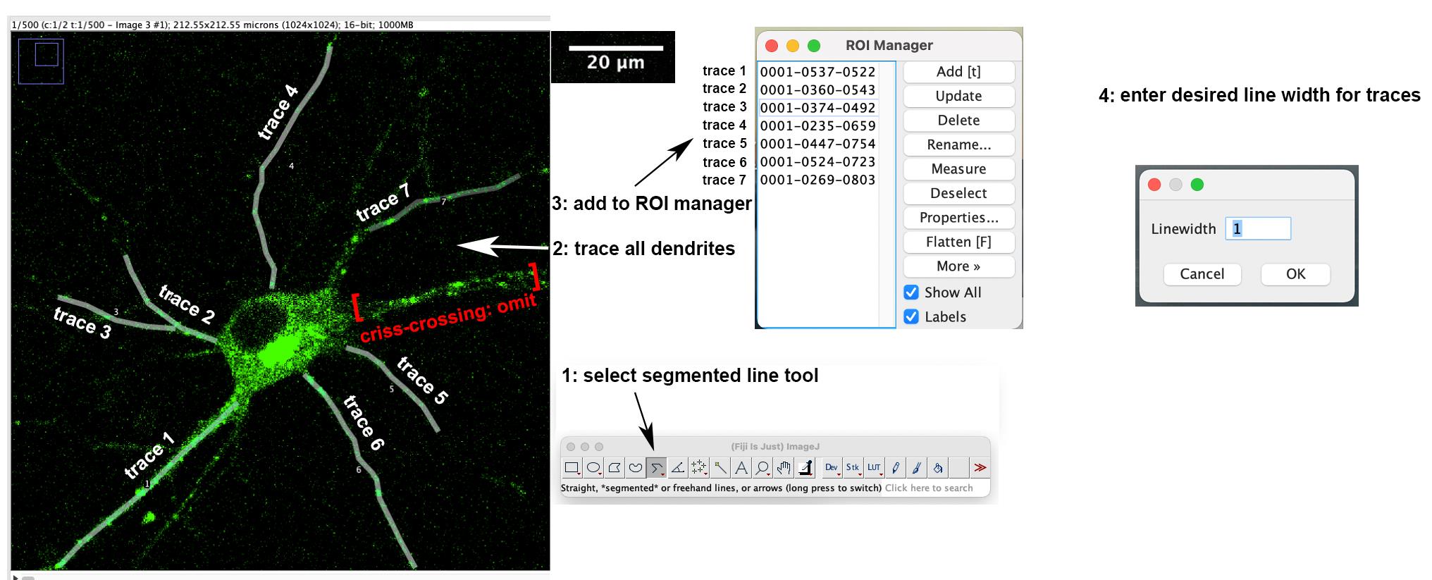
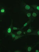
Figure 1. Tracing dendrites and adding to the ROI manager. Single plane image of the first time-lapse frame of a neuron transfected with GFP-RILP (Rab-interacting lysosomal protein) is shown. Dendrites are traced using the segmented line tool and added to the ROI manager. One trace is omitted because of crisscrossing dendrites.Once you are finished making the kymographs from the cell, save the image with the traced ROI on top of it. To do this, click Image > Overlay > From ROI Manager and then save as TIFF file for reference. This will allow you to go back to each cell at any point in the future and see which dendrite each kymograph came from.
Note: Potential problem—if there is bleaching during the imaging, use the bleach correcting plugin for FIJI (Miura, 2020; https://imagej.net/plugins/bleach-correction). If one experiences microscope stage drift during the imaging, a drift correction plugin exists in FIJI (https://imagej.net/plugins/manual-drift-correction).
Kymograph analysis
Multiple software packages exist. We have used manual analysis (Lasiecka et al., 2010 and 2014) as well as Kymograph Clear/Kymograph Direct software (Barford et al., 2018). These are briefly described in the Note below. Other programs exist and will also work.
Most recently, we have used KymoButler (Yap et al., 2022), a web-based software (Jakobs et al., 2019) available to customize with machine learning for a fee. A free version is available, which outputs velocities, track duration, and distances. https://www.wolframcloud.com/objects/deepmirror/Projects/KymoButler/KymoButlerForm. KymoButler is also available through a plugin for FIJI https://github.com/fabricecordelieres/IJ-Plugin_KymoButler_for_ImageJ.
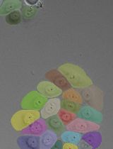
Analysis: KymoButler output can be customized to fit desired criteria for the questions of interest. For our purposes, KymoButler was customized to identify individual events and calculate data for each event, including speed, duration of movement or pausing, distance moved, or direction of movement. KymoButler also creates vesicle trajectories, which are comprised of multiple individual events. Data can be compiled for trajectories in addition to individual events. Creating trajectories from individual events can often not be accomplished for all vesicles for the entirety of the time-lapse imaging, but shorter unambiguous trajectories can usually be identified. In our experience, the trajectories created manually by a human user are almost identical to those created by KymoButler, since the same limitations exist for trajectory assignment by both (Figure 2).
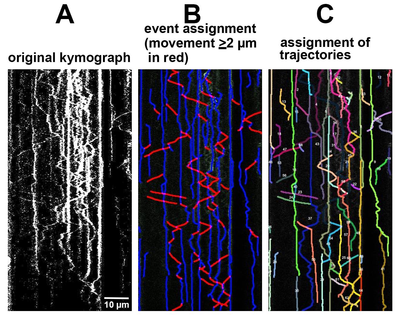
Figure 2. Software output for kymograph analysis. Original kymographs (A) are assigned events per user preference (for instance, defining motile events as ≥2 µm movements) (B) or trajectories (C). All events or trajectories identified by the software can be quantified in multiple ways, including speed, directionality, run lengths, or pause times.We have found it useful to use trajectory data to determine the net motility of individual vesicles over a longer time of the whole live imaging experiment instead of individual events. Net retrograde/anterograde/stationary data can be obtained from these measurements. For our purposes, we distinguished stationary trajectories (zero net movement) from short (<2 µm) and long (>2 µm) net movements. Theses cutoffs can be chosen by the user for their own questions. The raw data includes a full readout of distances traveled and can be binned into stationary vs. motile as per the user’s wishes. Since endosomes in dendrites pause and reverse direction a lot, we were more interested in the net behavior of vesicles and less interested in individual event measurements. For other questions, the user might be interested in individual event data. We create kymographs from all dendrites on any imaged cell for analysis (see Figure 1) and do not exclude dendrites unless they are not in focus or crisscrossing or bundling. We usually combine data from all the dendrites from one cell into one data point of motility data. So, the number of samples (n) for statistical purposes is usually one cell and not one dendrite or one vesicle. We find that imaging of ~20 cells (80–100 dendrites) gives good statistical power for endosome motility in dendrites. We recommend imaging at least 4–5 cells from 3–4 independent cultures and making kymographs from all dendrites for statistical analysis.
Note: We repeatedly trained the machine learning function of KymoButler on 20 kymographs for which ground truths had been established manually. Once the output from KymoButler closely matched the manual ground truth established by a human user, the same settings were used for all analyses. This initial training might need to be repeated for different types of fluorescent markers, because background haze might differ, and the same settings might not give satisfactory results. The event and trajectory assignments for each kymograph can be visually verified after KymoButler has finished to ensure accuracy.
Notes:
1. Manual analysis: Using the line tool in FIJI, manually trace all tracks on the kymograph and save them to the ROI manager as above. Using the known pixel size as determined from the objective and camera used, one can determine average velocities, retrograde and anterograde events, and pause events/times. This is laborious and time consuming, but the user has maximal control over the output. We usually validate software automation by comparing their output to manually established ground truth measurements for 10–20 kymographs.
2. Kymograph Clear/Kymograph Direct: open-source programs (Mangeol et al., 2016) available online for download and use with FIJI. These are sequential kymograph production and analysis programs that give user information regarding particle velocities, intensities, directionality, and run lengths. http://sites.google.com/site/kymographanalysis.
Double-channel kymograph: preparation and analysis
For generating double-channel kymographs, we created a plugin for ImageJ FIJI, called KymoMerge (currently only functional when using a Mac; McMahon et al., 2021).
Install KymoMerge: download from https://github.com/alduston/kymomerge. To begin using the merge tool, open FIJI and open the KymoMerge.py script in the FIJI console. The program can be installed as a plugin or run from the console.
Input the directory folders for the kymographs from each channel (Figure 3A).
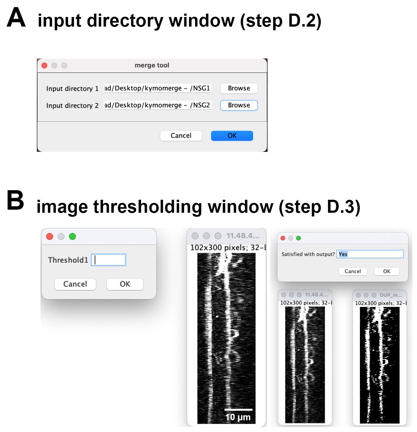
Figure 3. KymoMerge workflow. (A) Input directory window. This window will be used to choose the folders containing the kymographs from each channel. (B) Image thresholding window. This window will be used to input threshold values determined by the user for all images individually from each channel. Thresholding depends on the level of background fluorescence and the brightness of the signal. Each user needs to visually determine the optimal threshold value for their particular image.The files from each input directory (individual kymograph files) should have identical naming. Input directory should be a directory containing a series of named .tif files, using the naming convention ‘filename’-‘i’.tif, where i is the given .tif files ‘index’ in the folder. For instance, given three files in ‘groupA’ directory, using ‘kymo’ as file name, the .tif files would be given “kymo-1.tif, kymo-2.tif, kymo-3.tif.”
Input directory 2 should be a directory containing a series of named .tif files, using the naming convention ‘filename’-‘i’.tif, where i is the given .tif files ‘index’ in the folder. This index and file name should correspond to the index of input directory 1. The algorithm will compare files with corresponding indexes. For instance, given three files in ‘groupB’ directory, using ‘kymo’ as the file name as before, the .tif files would be given “kymo-1.tif, kymo-2.tif, kymo-3.tif.”
Kymograph image thresholding
The dialog box and image on the left comes up and shows the original kymograph along with an input to set the threshold (Figure 3B). The contrast for the original image is automatically increased so the data are clearly visible. When a value is chosen for the threshold by the user (typically 10–100 depending on background fluorescence and brightness of signal), the binarized image appears and can be compared to the original, as shown with the dialog box and images on the right. At this point, the user can accept the value by typing in Yes or choosing OK or try a new value by typing in No or choosing Cancel. Once a value is accepted, the next image opens. Once all images from the input folders are thresholded, they will be processed, and the output (individual binary images and merged image) will be available for further analysis as described above. Should the user want to quit the analysis at any point, simply type Quit into the dialog box.
Once the threshold is set, it is applied, and the image is converted to eight bits from the bit depth of the original image. This is then converted to a binary file and saved. Each pixel in the two channels is now set to a value of either 0 or 254.
Note: 8-bit images are used at this point because 16–32 bit formats interpolate locally to achieve greater color depth and make direct manipulation of individual pixel values more difficult.
The program then goes pixel by pixel between the two kymographs comparing values and creating a new image. If the values are both zero, or one is zero and the other is 254, the new image is set at zero at that pixel. If they are both 254 (positive signal in both channels), then the value is set at 254. The result is an image consisting only of those pixels where a positive signal is in both channels. This produces a kymograph containing tracks where the two proteins of interest are co-located, and the dynamics of the co-localized tracks can now be analyzed. The folder of co-located kymographs is saved in a new “output folder” in the folder containing the folder of original kymographs. The output folder contains the binarized kymographs from the input folders and the new, co-located kymograph. The program will open a file from the Group A directory of kymograph files (channel 1) for the user to threshold, followed by the corresponding file from the Group B directory (channel 2). This will continue until all the images are thresholded.
Notes
KymoMerge vs. manual kymograph analysis
Two sample data sets are used to test and validate the reliability and efficiency of the program. One consists of the neuronal membrane proteins NSG1-cherry and NSG2-GFP. NSG1 and NSG2 are members of a neuron-specific gene family of proteins. Both proteins are highly expressed in neurons and localized to a variety of endosomal compartments in dendrites (Yap et al., 2017). Our previous live imaging data showed that both proteins co-trafficked in neurons, and thus serve as a good example for analyzing the dynamics of two highly co-localized membrane cargos with low background noise signals (Figure 4A). The second data set contains NSG1-cherry with GFP-RAB7, a late endosome marker. RAB7 is a small GTPase involved in regulating transport to late endocytic compartments. We have previously shown that RAB7 co-trafficked and regulated the endocytic transport of NSG1 in neurons (Yap et al., 2017). Like other Rabs, RAB7 is constantly cycling between the activated form (GTP-bound) when it is recruited to membranes and inactivated form (GDP-bound) after hydrolysis and when it is cytosolic. This feature allows us to test the ability of our program in extracting membrane-bound signals from cytosolic high background signals (Figure 4C).
Visualizing co-localized tracks
In Figure 4, we give examples of typical output from KymoMerge. Figure 4A shows kymographs from the NSG1 and NSG2 data set with NSG1 in red and NSG2 in green, while Figure 4C shows example kymographs from the GFP-RAB7 and NSG1-mcherry data set. The top row shows the original 32-bit single-channel images followed by an overlay of the two channels. Below are the binary outputs from KymoMerge. Careful comparison of the original images in Figure 4A, C with the binary output of KymoMerge (Figure 4B and 4D) shows very similar tracks between the two. Due to the binary nature of the KymoMerge output, it does not show intensity differences as in the original files, but this is not a parameter that is usually of interest in kymograph analysis. Intensity differences are only used initially in determining background levels and true signal during the thresholding stage before the binary output is created. Comparison of the overlayed and merged files also shows similar characteristics.
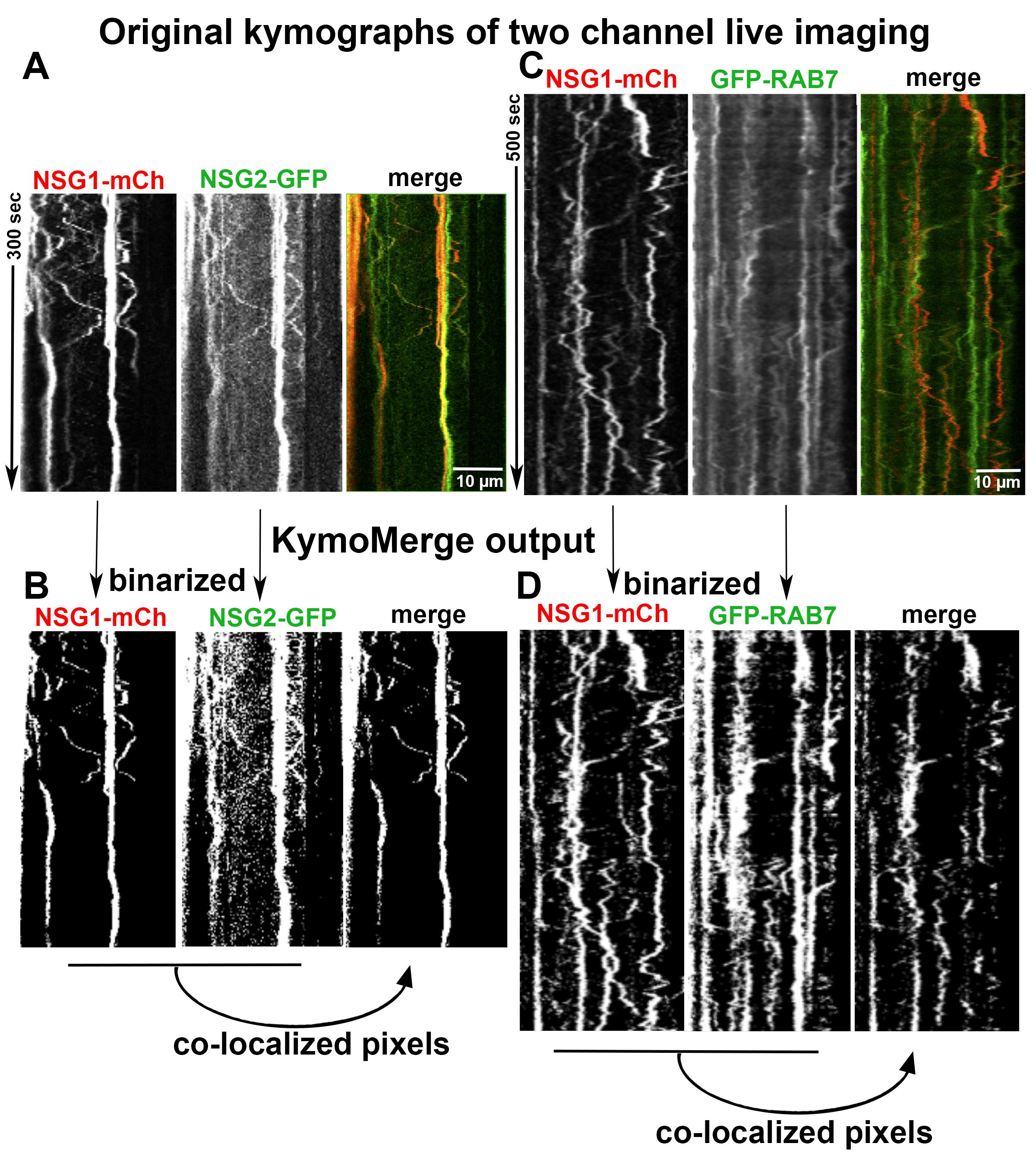
Figure 4. Comparison of original images vs. KymoMerge-generated images. Dual live imaging was carried out for two transmembrane proteins, NSG1-mCh and NSG2-GFP (A and B), and for NSG1-mCh with a cytosolic regulator GFP-RAB7 (C and D). The original kymographs for each channel and a merged kymograph are shown in (A) and (C). The binarized single-channel kymographs created by KymoMerge are shown in (B) and (D), together with the co-localized output kymograph. This final output of co-localized pixels can be used for further quantitative analysis.One of the principal strengths of our approach is that any track seen in the merged binary data is a co-located track. In contrast, it can be difficult to discern coincident tracks in the original data.
Testing the robustness of KymoMerge
Our approach is useful only if the program produces results that are robust and reliable. We find that KymoMerge produces results comparable to those from a careful count done by hand, which is often how kymograph data is analyzed. For this purpose, we took the two data sets referenced in Figure 4A, B and 4C, D and independently counted anterograde and retrograde events (≥ 2 μm) manually, referencing either the original and overlayed data (as shown in Figure 4A and 4C) or using the merged binary output from KymoMerge (as shown in Figure 4B and 4D). The results in Figure 5A and 5B show that there was no statistical difference between the two methods (Mann-Whitney test).
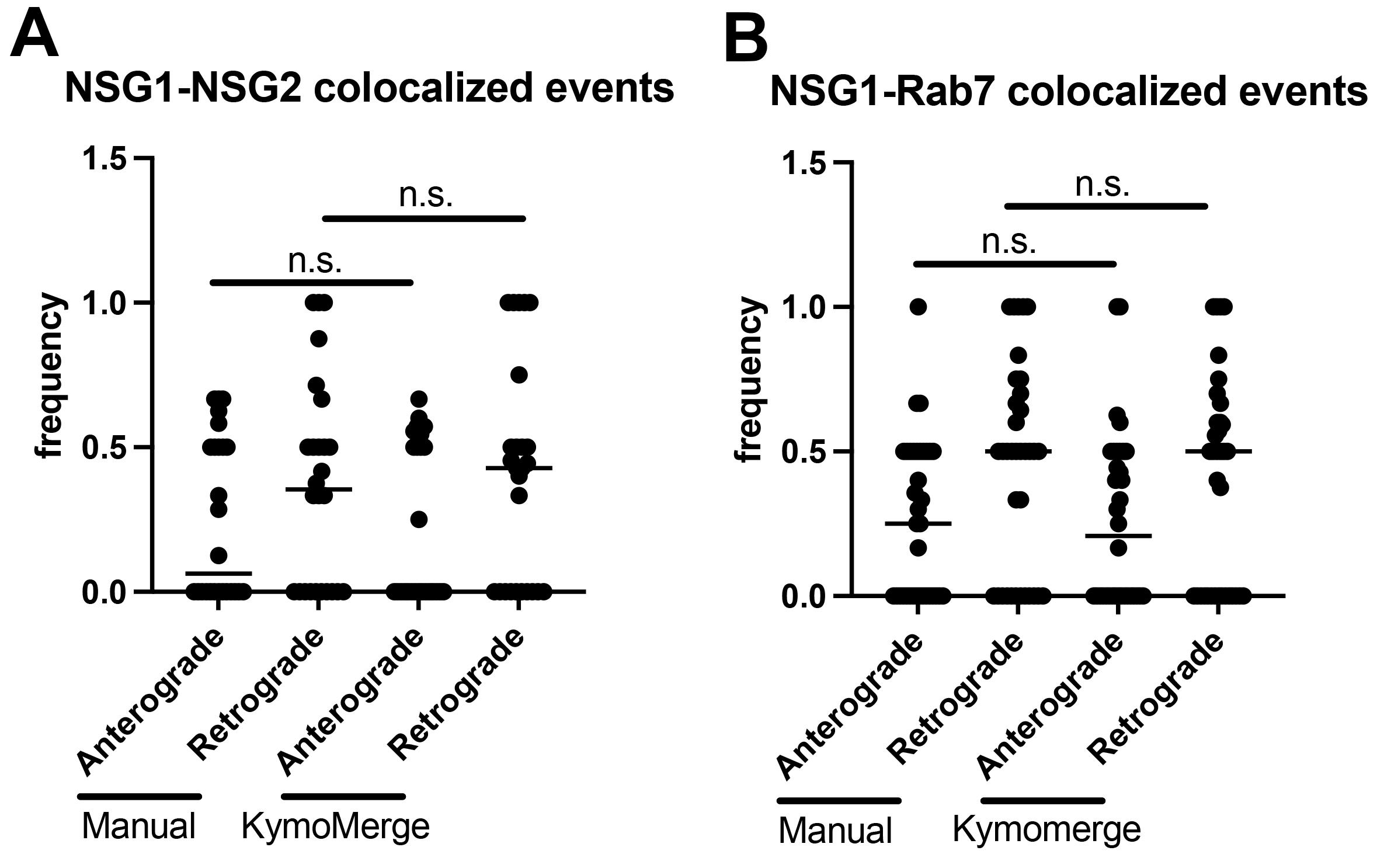
Figure 5. Comparison between manual counts of anterograde and retrograde events (≥ 2 μm) using original 32-bit images and KymoMerge created kymographs. (A) n = 26 dendrites from seven neurons in the NSG1-mCherry/NSG2-GFP data set. (B) n = 36 dendrites from seven neurons in the NSG1-mCherry/GFP-RAB7 data set. Statistical results from Mann-Whitney test between anterograde or retrograde pairs.Caveats on binary thresholding
Thresholding of images is often necessary in image analysis, but it can also be somewhat subjective and, therefore, potentially problematic. With KymoMerge, thresholding requires attention particular to the process of creating binary images. There is a difficulty inherent to the process of creating the binary images: if one region is noisier than another, the noise can be of the same magnitude as the signal elsewhere. The result is that the set threshold will either eliminate actual signal if it is at a level suitable for the noisier regions, or potentially background will be left, creating false co-localized tracks. Careful thresholding with KymoMerge can produce an accurate and interpretable merged kymograph. For kymographs with areas of high background, it may be necessary to crop excessively noisy areas before analysis. Since these areas would generally be uninterpretable even with manual analysis, analyzable data are not being lost and the rest of the image will produce accurate results. It is important to understand that any data set is only a sampling of the system being studied. It is better to err on the side of excluding false positive co-localized tracks and analyze only the resulting tracks that are truly co-localized. Because KymoMerge allows for individual screening and thresholding of the individual channels before the merged images are created, any problematic kymographs can be identified by the user and properly processed. More examples are shown in McMahon et al. (2021), including direct comparisons of two different thresholds used on the same data sets.
Acknowledgments
This research was supported by NIH R01NS083378. The initial publication where this method is published: Yap et al. (2022).
Competing interests
No competing financial interests for this study.
Ethics
Neuronal cultures used for live imaging were prepared from E18 rat embryos as approved by the University of Virginia Animal Care and Use Committee. All experiments were performed in accordance with relevant guidelines and regulations (ACUC #3422).
References
- Barford, K., Keeler, A., McMahon, L., McDaniel, K., Yap, C. C., Deppmann, C. D. and Winckler, B. (2018). Transcytosis of TrkA leads to diversification of dendritic signaling endosomes. Sci Rep 8(1): 4715.
- Boecker, C. A., Olenick, M. A., Gallagher, E. R., Ward, M. E., Holzbaur, E.L.F. (2020). ToolBox: Live Imaging of intracellular organelle transport in induced pluripotent stem cell-derived neurons. Traffic 21: 138-155.
- Chien, A., Shih, S. M., Bower, R., Tritschler, D., Porter, M. E. and Yildiz, A. (2017). Dynamics of the IFT machinery at the ciliary tip. Elife 6: e28606.
- Farías, G. G., Guardia, C. M., De Pace, R., Britt, D. J. and Bonifacino, J. S. (2017). BORC/kinesin-1 ensemble drives polarized transport of lysosomes into the axon.Proc Natl Acad Sci U S A 114(14): E2955-E2964.
- Farfel-Becker, T., Roney, J. C., Cheng, X. T., Li, S., Cuddy, S. R. and Sheng, Z. H. (2019). Neuronal Soma-Derived Degradative Lysosomes Are Continuously Delivered to Distal Axons to Maintain Local Degradation Capacity. Cell Rep 28(1): 51-64.
- Ganguly, A. and Roy, S. (2022). Imaging Diversity in Slow Axonal Transport. Methods Mol Biol. 2431:163-179.
- Hertzler, J. I., Simonovitch, S. I., Albertson, R. M., Weiner, A. T., Nye, D. M. R. and Rolls, M. M. (2020). Kinetochore proteins suppress neuronal microtubule dynamics and promote dendrite regeneration. Mol Biol Cell 31(19): 2125-2138.
- Jakobs, M. A., Dimitracopoulos, A. and Franze, K. (2019). KymoButler, a deep learning software for automated kymograph analysis. Elife 8: e42288.
- Lasiecka, Z. M., Yap, C. C., Caplan, S. and Winckler, B. (2010). Neuronal early endosomes require EHD1 for L1/NgCAM trafficking. J Neurosci 30(49): 16485-16497.
- Lasiecka, Z. M., Yap, C. C., Katz, J. and Winckler, B. (2014). Maturational conversion of dendritic early endosomes and their roles in L1-mediated axon growth.J Neurosci 34:14633.
- Lasiecka, Z. M. and Winckler, B. (2016). Studying endosomes in cultured neurons by live-cell imaging. In K. K. Pfister (Ed.), The Neuronal Cytoskeleton, Motor Proteins, and Organelle Trafficking in the Axon. Methods in Cell Biology 131:389-408.
- Liang, X., Kokes, M., Fetter, R. D., Sallee, M. D., Moore, A. W., Feldman, J. L. and Shen, K. (2020). Growth cone-localized microtubule organizing center establishes microtubule orientation in dendrites. Elife 9: e56547.
- Maday, S. and Holzbaur, E. L. (2016). Compartment-Specific Regulation of Autophagy in Primary Neurons. J Neurosci 36(22): 5933-5945.
- Mangeol, P., Prevo, B. and Peterman, E. J. (2016). KymographClear and KymographDirect: two tools for the automated quantitative analysis of molecular and cellular dynamics using kymographs. Mol Biol Cell 27(12): 1948-1957.
- McMahon, L. P., Digilio, L., Duston, A., Yap, C. C. and Winckler, B. (2021). KymoMerge: a new tool for analysis of multichannel kymographs. BioRxiv doi: https://doi.org/10.1101/2021.11.29.470387
- Menon, M., Askinazi, O. L. and Schafer, D. A. (2014). Dynamin2 organizes lamellipodial actin networks to orchestrate lamellar actomyosin. PLoS One 9(4): e94330.
- Miura, K. (2020). Bleach correction ImageJ plugin for compensating the photobleaching of time-lapse sequences. [version 1]. F1000Res 9: 1494.
- Wang, X. and Schwarz, T. L. (2009). Chapter 18: Imaging Axonal Transport of Mitochondria.Methods Enzymol 457: 319-333.
- Yap, C. C., Wisco, D., Kujala, P., Lasiecka, Z. M., Cannon, J. T., Chang, M. C., Hirling, H., Klumperman, J. and Winckler, B. (2008). The somatodendritic endosomal regulator NEEP21 facilitates axonal targeting of L1/NgCAM. J Cell Biol 180(4): 827-842.
- Yap, C. C., Digilio, L., McMahon, L. and Winckler, B. (2017). The endosomal neuronal proteins Nsg1/NEEP21 and Nsg2/P19 are itinerant, not resident proteins of dendritic endosomes. Sci Rep 7(1): 10481.
- Yap, C. C., Digilio, L., McMahon, L. P., Garcia, A. D. R. and Winckler, B. (2018). Degradation of dendritic cargos requires Rab7-dependent transport to somatic lysosomes. J Cell Biol 217(9): 3141-3159.
- Yap, C.C., Digilio, L., McMahon, L.P., Wang, T. Winckler, B. (2022). Dynein Is Required for Rab7-Dependent Endosome Maturation, Retrograde Dendritic Transport, and Degradation. J Neurosci 42(22): 4415-4434.
- Zwetsloot, A. J., Tut, G. and Straube, A. (2018). Measuring microtubule dynamics. Essays Biochem 62(6): 725-735.
Article Information
Copyright
© 2023 The Author(s); This is an open access article under the CC BY-NC license (https://creativecommons.org/licenses/by-nc/4.0/).
How to cite
Readers should cite both the Bio-protocol article and the original research article where this protocol was used:
- Laura, D., McMahon, L. P., Duston, A., Yap, C. C. and Winckler, B. (2023). Quantifying Single and Dual Channel Live Imaging Data: Kymograph Analysis of Organelle Motility in Neurons. Bio-protocol 13(10): e4675. DOI: 10.21769/BioProtoc.4675.
- Yap, C.C., Digilio, L., McMahon, L.P., Wang, T. Winckler, B. (2022). Dynein Is Required for Rab7-Dependent Endosome Maturation, Retrograde Dendritic Transport, and Degradation. J Neurosci 42(22): 4415-4434.
Category
Neuroscience > Cellular mechanisms
Cell Biology > Cell imaging > Live-cell imaging
Do you have any questions about this protocol?
Post your question to gather feedback from the community. We will also invite the authors of this article to respond.