- Protocols

- Articles and Issues
- For Authors
- About
- Become a Reviewer

Fast Detection and Quantification of Interictal Spikes and Seizures in a Rodent Model of Epilepsy Using an Automated Algorithm
(*contributed equally to this work) Published: Vol 13, Iss 6, Mar 20, 2023 DOI: 10.21769/BioProtoc.4632 Views: 2108
Reviewed by: Prashanth N SuravajhalaJayaraman ValadiWenyang LiAnonymous reviewer(s)
Original research article
The authors used this protocol in:

Aug 2022
Advertisement


Protocol Collections
Comprehensive collections of detailed, peer-reviewed protocols focusing on specific topics


Related protocols
Abstract
The electroencephalogram (EEG) is a powerful tool for analyzing neural activity in various neurological disorders, both in animals and in humans. This technology has enabled researchers to record the brain’s abrupt changes in electrical activity with high resolution, thus facilitating efforts to understand the brain’s response to internal and external stimuli. The EEG signal acquired from implanted electrodes can be used to precisely study the spiking patterns that occur during abnormal neural discharges. These patterns can be analyzed in conjunction with behavioral observations and serve as an important means for accurate assessment and quantification of behavioral and electrographic seizures. Numerous algorithms have been developed for the automated quantification of EEG data; however, many of these algorithms were developed with outdated programming languages and require robust computational hardware to run effectively. Additionally, some of these programs require substantial computation time, reducing the relative benefits of automation. Thus, we sought to develop an automated EEG algorithm that was programmed using a familiar programming language (MATLAB), and that could run efficiently without extensive computational demands. This algorithm was developed to quantify interictal spikes and seizures in mice that were subjected to traumatic brain injury. Although the algorithm was designed to be fully automated, it can be operated manually, and all the parameters for EEG activity detection can be easily modified for broad data analysis. Additionally, the algorithm is capable of processing months of lengthy EEG datasets in the order of minutes to hours, reducing both analysis time and errors introduced through manual-based processing.
Background
The emphasis of translational research in epilepsy is now shifting from the development of anti-seizure therapies to anti-epileptogenic and disease-modifying treatments. Long-term electroencephalographic recordings during the acute and chronic phases of disease are an important part of the drug-testing paradigm for these therapies. Manual analysis of prolonged electroencephalography (EEG) recordings can be time-consuming, laborious, and expensive. Further, manual EEG interpretation risks the introduction of human error and implicit bias, which can negatively impact data quantification and subsequent findings (Arends et al., 2017; Benbadis et al., 2017; Barger et al., 2019). Improper EEG analysis generates inconsistent data, which skews interpretation of the efficacy of interventional therapies at preventing the advent or progression of disease. Additionally, the limited signal-to-noise ratio makes manual analysis of seizures, seizure patterns, epileptiform spikes, and detection of other epileptiform events extremely challenging (Kaplan et al., 2005; Liu et al., 2019). These issues present a sizeable roadblock to rapid and unbiased scoring of electrographic spikes and seizure analysis. An automated, algorithm-based EEG analysis program is an ideal solution to meet this goal.
Previous work towards the development of automated EEG analysis tools has led to the production of algorithms that are capable of detecting and quantifying interictal activity and seizures, both in real-time and post data collection (Bergstrom et al., 2013;Tieng et al., 2016 and 2017). Unfortunately, many of these algorithms have been produced in programming languages that are no longer widely used or require substantial computational power to operate effectively (Harner et al., 2009). As a result of the steady evolution in the capabilities of computer processing equipment, higher levels of computational power can now be achieved. However, these new computational technologies are expensive, and often require additional hardware upgrades to be utilized in computing systems. Therefore, we developed an algorithm that detects and quantifies interictal spikes and seizures, using a programming language that requires minimal computational power and a computer with average processing hardware.
We evaluated our novel spike detection algorithm—a Basic Function Algorithm programmed in MATLAB—using large-scale EEG data obtained from a mouse model of epilepsy. We utilized EEG traces from mice with traumatic brain injury–induced epilepsy. The interictal spikes and seizures were manually detected using commercially available software (Neuroscore, Data Science International), and automatically detected using our EEG algorithm. All seizures detected using the automated algorithm were cross-referenced with Neuroscore for verification. Our comparative analysis revealed that the automated, algorithmic scoring of electrographic spikes and seizures is faster, more accurate, and less laborious than manual EEG analysis. Moreover, the algorithm is more dependable, resulting in a lower risk of introducing bias than manual, visual-based analysis.
Materials and Reagents
Materials for electrode implantation
Forceps, scalpel handles, scissors (Stoelting, catalog numbers: 5210883P, 52171P, 5210002P)
26 Gauge needles (Fisher Scientific, catalog number: BD 305111)
1 mL syringes (Fisher Scientific, catalog number: BD 309659)
Cotton tip applicators (Puritan, catalog number: 806 WC)
Burr drill tips (Stoelting, catalog number: 514552)
Surgical clips (Cellpoint Scientific, catalog number: 203-1000)
Surgical sutures, size 5-0 (Ethicon, catalog number: J493G)
Dental cement (Co-Oral-ite MFG Co, catalog number: 525000)
HD-X02 implants with two biopotential channels [Data Sciences International (DSI) (division of Harvard Bioscience, Inc)], catalog number: 270-0172-001)
Reagents
70% ethanol
Chlorhexidine scrub (Mölnlycke, catalog number: 0234-0575-08)
0.9% saline solution
Artificial tears ointment (Aventix, catalog number: 13585)
Meloxicam (Norbrook, catalog number: 0342.90A)
Baytril (Bayer Pharmaceuticals LLC, catalog number: AH039GH)
5% Haemo-Sol regular (Haemo-Sol, catalog number: 026-050)
Equipment
EEG acquisition system
Ponemah Software System (DSI, catalog number: PNM-P3P-CFG)
Included in system:
Analysis Module – Electroencephalogram Analysis Software Module (PNM-EEG100W)
Video Module – Noldus media recorder (PNM-VIDEO-008)
Ponemah Software 6.51 (PNM-P3P-651)
New Ponemah Acquisitions Software (PNM-P3P-TELELV8)
Analysis Module – Electromyogram Analysis Software module (PNM-EMG100W)
Computer – Lenovo ThinkPad T490 64-bit Windows 10 with docking station (271-0112-031)
Small Business Router – Cisco RV160 VPN router (DSI, catalog number: RV160)
Network Switch – 183w Network Switch (DSI, catalog number: 271-0115-003)
MX2 – Matrix 2.0 with USB Port for Signal Interface Support (DSI, catalog number: 271-0119-002)
RPC-1 – Receiver Pad for Plastic Cages with 4.5 m cable (DSI, catalog number: 272-6001-001)
Neuroscore software (DSI, 271-0165-CFG)
Included in system:
NS 3.3 Core – Neuroscore v3.3 Core software (271-0165-330)
Seizure Module – Neuroscore Seizure module (271-0167-SEIZURE)
Video Module – Neuroscore Video Synchronization module (271-0168-VIDEO)
Video Camera – Axis M1145-L Network Camera Kit with Axis T8120 Midspan (AXIS, catalog number: 275-0204-001)
Computational hardware
One of the primary goals of this project was to develop an autonomous algorithm that could rapidly process large volumes of EEG data using minimal computational power. To do so, an HP Spectre x360 laptop (Manufacturer: HP, Model: 15-eb1043dx) was used to process all EEG data. The CPU utilized was an Intel i7-10510U running at 2.30 GHz base clock speed, with a maximum clock speed of 4.30 GHz on all four cores. A total of 16 GB of GDDR4 memory was operated at 2667 MHz. The laptop had an additional 32 GB of Intel Optane memory available; however, this was disabled during data processing, and thus the maximum memory available at any given time was 16 GB. The laptop contained an Nvidia MX250 graphics card; however, since MATLAB is a CPU-intensive program, GPU processing power was not strongly considered. EEG data was written on an internal M.2 solid-state drive, after increased processing times were observed when using a standard USB 2.0 hard disk drive.
Software
Windows 10 Operating System (Microsoft, https://www.microsoft.com/en-us/software-download/windows10)
Neuroscore, Version 3.3 (Data Sciences International, https://www.datasci.com/products/software/neuroscore)
Ponemah Software 6.51 (https://www.datasci.com/products/software/ponemah)
MATLAB R2021a (MathWorks, https://www.mathworks.com/products/matlab.html)
MATLAB Signal Processing Toolbox (MathWorks, https://www.mathworks.com/products/signal.html)
Procedure
In the following sections, we describe the procedures for electrode implantation, EEG acquisition, and analysis of interictal spikes and seizures. For more information on electrode implantation and EEG acquisition procedures, we direct readers to the original articles (Puttachary et al., 2015; Sharma et al., 2018 and 2021).
Surgical preparation and electrode implantation
Clean surgical equipment with 5% Haemo-Sol solution for 48–72 h and dry at room temperature prior to autoclaving. On the day of surgery (electrode implantation), shave each mouse’s head (under anesthesia), and clean the surgical site in an onion shell pattern with 70% ethanol and a chlorhexidine scrub. Administer analgesic (Meloxicam, 1–2 mg/kg, subcutaneous) and eye ointment prior to surgery. Using a scalpel, make a small midline incision at the mid-dorsal aspect of the head and neck. Insert a transmitter into the flank region, by tunneling between the skin and the fascia using blunt dissection. Then, drill bilateral holes into the skull of each hemisphere, and place electrodes epidurally into the cerebral hemispheres. Completely cover and secure the electrodes in place using dental cement. Close the incision using sterile surgical sutures (Puttachary et al., 2015; Sharma et al., 2018 and 2021).
A video of the electrode implantation protocol has been provided (Video 1).
 Video 1. Mouse electrode implantation procedure
EEG acquisition and setup
PhysioTelTM radio telemetry devices (transmitters) use oscillators controlled by voltage that convert biopotentials into high-frequency signals. All PhysioTelTM HD radiotelemetric devices are equipped with serial numbers. Once turned on, these devices send signals to receiver pads that record the serial number from the implanted device. These high-frequency signals are then transferred to the data exchange matrix that forwards output signals to the computer. Eight receiver pads can be connected to a single data exchange matrix, and multiple video-synchronized EEG traces can be monitored simultaneously through Ponemah Software 6.51, with a sampling frequency of 1,000 Hz. All information regarding the receiver pads, animal identification number, transmitter serial number, jack location in the data matrix, signal strength, and transmitter information, such as EEG and temperature calibration, are recorded to each matrix under hardware settings in the acquisition window. The acquisition of the EEG signal is performed at a sampling rate of 1,000 Hz, filter cutoff at 100 Hz, and full scale at 10 mV, by the Ponemah Acquisition Software. The frequency range of the telemetry transmitter is 1–100 Hz. Shortly after the implantation of the transmitters, start EEG recording to obtain baseline activity tracings for each animal. Approximately 5 GB of video (at 20 frames/s) and EEG data can be collected per day from eight animals simultaneously (Puttachary et al., 2015; Sharma et al., 2018). Once data acquisition is complete, export the EEG data as EDF files, to be used within MATLAB.
Installation of MATLAB and toolboxes
MATLAB can be installed from the MathWorks product webpage for Windows, Linux, and Macintosh operating systems (OS). For our purposes, a Windows OS was used, and the following instructions pertain to installation of MATLAB on a Windows 64-bit OS. However, additional information regarding MATLAB installation on a Linux OS can be found in the Notes section. First, create a MathWorks account and navigate to https://www.mathworks.com/products/matlab.html to view available products. Select the version of MATLAB you wish to download and click “Download for Windows.” Open the installation file by double clicking on it once it has downloaded. Sign in to your MathWorks account when prompted and follow the on-screen instructions to finish installation. During installation, select the MathWorks Signal Processing Toolbox and install the supplemental software package when prompted, to select add-on applications.
Manual EEG Analysis
Electrographic spikes and seizures are first detected manually using Neuroscore 3.3 software, which is commercially available from DSI. Spikes are analyzed using the “spike train protocol,” which identifies epileptiform spikes and spike duration, using dynamic and absolute threshold values. Dynamic thresholding allows a user to define a threshold based on a multiplication of the root mean square value of the EEG signal approximately one minute prior to the time point being analyzed, while the absolute threshold allows the user to define a fixed amplitude threshold (voltage) that is applied in both the positive and negative directions. Dynamic threshold values include threshold ratio as well as maximum and minimum ratios for epileptiform spike detection–criteria, which prevent false positives from being detected in low noise settings. The absolute threshold values include minimum and maximum amplitudes for EEG spikes, which are kept between 200 and 1,500 μV. Therefore, all spikes above 200 μV are considered epileptiform spikes. These parameters are specified to extract epileptiform spikes from the raw EEG data. These parameters also consider the minimum and maximum time interval between spikes, which is used to determine possible members of a spike train. Lastly, the duration of a spike train is also used to filter true epileptiform activity from background noise. Once the settings are finalized, load the raw EEG data via the EDF file, and specify the required signals (power bands and activity counts). Once complete, the raw EEG file can be analyzed (Puttachary et al., 2015). Interictal spikes and seizures are differentiated based on the EEG spike characteristics, such as amplitude, inter-spike interval, duration, and power spectral analysis. Manually remove EEG signals associated with mouse behavior (exploratory and grooming) and electrical artifacts, so they do not interfere with the analysis. These behavioral activities can be verified via video EEG recordings (Tse et al., 2014; Puttachary et al., 2015).
For seizure analysis, we set the duration for seizures (CS) at >10 s. CS episodes can last from 10–120 s, with inter-spike intervals of 100–300 ms. Spike amplitude often varies from 500–1,500 μV, with a spike frequency/min of 180–720 within an episode (Puttachary et al., 2015). Additionally, the power band spectrum is known to be a reliable measure for the detection of seizures (Puttachary et al., 2015; Sharma et al., 2018). The power spectrum varies with the type of seizure, and the spectrum frequently changes within stage-specific seizures (Tse et al., 2014; Puttachary et al., 2015).
Algorithm-based (automated) EEG analysis
File path and data import (Block 1)
The MATLAB EEG algorithm was programmed using three grouped blocks of code. The first block of the algorithm establishes a file path to the working folder and imports all the EDF files present within that folder using the edfread function. This allows the user to extract every EDF file using a single button click. Once imported, the EEG data from the EDF files is stored within cell arrays, using the default units of seconds and microvolts (μV). The algorithm then converts the EEG amplitude values into millivolts (mV). Then, the recording date is converted into a date-number format, while the time values are converted from a frequency value to a whole number in seconds.
Baseline EEG activity determination (Block 2)
The second block of code contains the data processing elements, allowing the algorithm to autonomously locate and record the location of interictal spikes and seizures. First, the algorithm calculates the baseline EEG activity value via a “running while” loop. This is done by iterating from a set minimum of 100 μV by increments of 5 μV, until 97% of the baseline EEG data points in the first hour of data are less than the value of the current iteration. Once this condition is satisfied, the algorithm saves the current amplitude iteration, outputs the value on-screen to the user, and proceeds with the calculation of the upper and lower spike thresholds. The time window (default ~1 h) for determining baseline activity can be readily changed from 1 h to any value that is suitable for the user, as long as it is shorter than the total length of the EEG tracing. This modification allows users to analyze EEG traces that are less than 1 h long and provides the opportunity to achieve a more accurate baseline by extending the time window beyond 1 h, if needed.
Lower threshold and upper threshold determination (Block 2)
The lower threshold variable incorporated in the algorithm is the value at which a true interictal spike is differentiated from background EEG noise and normal baseline activity. Relevant literature has revealed that a lower threshold of twice the baseline activity value is often sufficient for differentiating true interictal activity from the baseline EEG signal (Anjum et al., 2018). After determining baseline EEG activity, as described in the previous section, the algorithm calculates the lower threshold for interictal differentiation by doubling the baseline activity value. Thus, the lower threshold value for interictal spiking is not fixed, but rather depends on the baseline activity value of each individual EEG tracing. The upper threshold for interictal spiking is also pre-specified, to differentiate true interictal spikes from background electrical noise or animal movement. As reported in the literature, an upper threshold value of 1,500 μV often accurately captures true interictal activity, while removing EEG artifacts due to noise and animal behavior (Tse et al., 2014; Puttachary et al., 2015; Casillas-Espinosa et al., 2019). The upper threshold value is fixed, for every EEG trace, but can be readily adjusted as needed.
Interictal spike detection (Block 2)
Following determination of these key parameters, the remainder of the second block of code detects interictal spikes and seizures. The algorithm detects EEG spikes using the findpeaks function that is part of the MathWorks Signal Processing Toolbox, alongside a variety of associated input arguments used to clarify interictal activity. The minimum distance between interictal spikes, MinPeakDistance, is set at a value of 100 ms, to ensure that poly-spikes and other abnormal spiking patterns are not counted as multiple spikes (Puttachary et al., 2015). The minimum peak prominence, MinPeakProminence, better described as relative peak amplitude, is set at a value of 200 μV, which is also used to reduce the detection of poly-spikes and abnormal activity, such as grooming and mouse movement. Minimum peak amplitude, MinPeakHeight, is specified at the lower threshold value to ensure that only spikes with twice the baseline activity value are counted as interictal spikes. Lastly, a maximum peak width, MaxPeakWidth, of 200 ms is specified to reduce quantification of abnormal spikes and EEG artifacts. As with other quantification parameters, all these values are easily modified to filter the EEG trace being analyzed. After completing interictal spike detection, the algorithm records the date, time, and amplitude of every interictal spike that has met all the prespecified constraints, and provides the option to generate on-screen figures, as in Figure 1. Then, the algorithm removes any spike that fails to meet all the specified criteria (Table 1) from further quantification.

Figure 1. Representative example of interictal spikes determined using the automated algorithm. (A) MATLAB-generated output showing interictal activity detection (positive and negative spikes marked by red circles). The blue horizontal lines represent the automatically determined baseline activity value and the red horizontal lines represent the lower threshold value (2X baseline activity). (B) An enlarged image of an individual inter-ictal spike.Table 1. Criteria for determining the presence of interictal spikes for algorithmic analysis
Interictal Spike Classification Criteria Lower Detection Threshold 2X Baseline Activity Value Upper Detection Threshold ≤1,500 μV Minimum Peak Prominence ≥200 μV Maximum Peak Width 200 mS Inter-spike Interval ≥100 mS Seizure detection (Block 2)
The last section of code in the second block contains the seizure detector, which analyzes the EEG trace subsequent to the interictal spike quantification process described in the previous section. Seizures are defined as an electrographic seizure with high amplitude frequency discharges, lasting for at least 10 seconds (Guo et al., 2013; Goodrich et al., 2013), with three times the baseline activity value, and an inter-spike interval of less than 5 seconds (Puttachary et al., 2015). The criteria for quantifying seizures are based on published literature quantifying spike clusters and grouped ictal activity for the evaluation of epileptogenesis (Tse et al., 2014; Puttachary et al., 2015; Anjum et al., 2018; Casillas-Espinosa et al., 2019). First, using the data from the previous section of code, the algorithm calculates the time elapsed between adjacent electrographic spikes. The algorithm then determines the starting and ending points of clusters of spiking activity. Any interval that is greater than the prespecified 5-second inter-seizure interval will break the chain of spiking activity, and automatically restart quantification of the next cluster of activity. Once complete, the code processes each spike cluster and removes any cluster that fails to meet the predefined seizure criteria (Table 2). If all the criteria are met, the algorithm stores these ictal activity clusters as well as the corresponding date, time of onset, duration, and number of ictal spikes within the cluster, which can be plotted for on-screen analysis (Figure 2).
Table 2. Criteria for determining the presence of a seizure during algorithmic analysis
Seizure Classification Criteria Minimum Spike Amplitude 3X Baseline Activity Value Maximum Spike Amplitude ≤1,500 μV Minimum Seizure Duration >10 s Maximum Inter-Spike Interval <5 s 
Figure 2. Visual representation of spike and seizure detection within MATLAB. (A) Segment of the EEG trace showing interictal events and seizures on day 21 post-injury. Three episodes of spontaneous seizures were observed on the same day in one mouse (shown in rectangular blocks marked with triangles). (B) Expanded EEG trace of one of the seizures from 'A'. (C) Increased EMG activity is shown below the seizure trace. (D) Further expanded EEG trace of the seizure shown in C. Abbreviations: IIE, interictal events; EEG, electroencephalogram; EMG, electromyogram; SRS, spontaneous recurrent seizures.Data Processing and Export (Block 3)
The third and final block of code is responsible for terminal data processing, and exporting compiled data to Microsoft Excel, for further data manipulation or comparison. First, there are instructions for plotting data so the data can be viewed on-screen, if desired. To reduce the computational workload and promote time savings, the plotting instructions are suppressed by default. However, in the semi-automated version of the code, plotting is displayed on-screen, allowing the user to manually review each interictal spike and seizure. The remaining code creates individual data tables containing the interictal spike data and seizure data for each EEG file present in the current working folder. Thus, when the code terminates, the interictal spike counts and seizure quantification data for all EEG traces are written to separate Excel files and stored within the current folder. This allows the user to rapidly process multiple EEG traces and have the data readily available for further review, or further analysis outside the MATLAB programming environment. Figure 3 provides a simplified, graphical representation of the various algorithm blocks and processing steps.
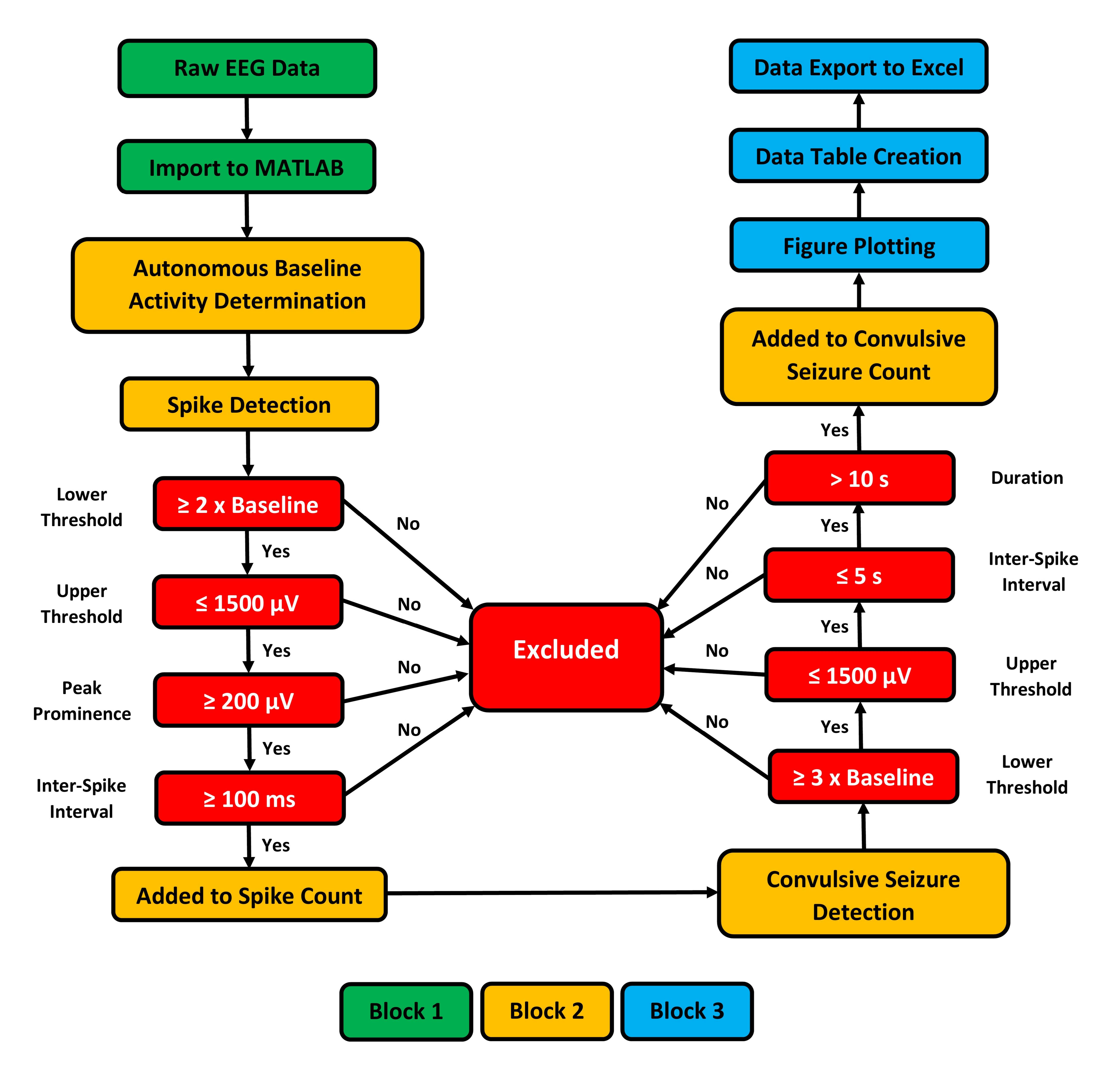
Figure 3. Schematic diagram outlining the processing steps of the autonomous MATLAB algorithm created for the detection of interictal spikes and seizures. Block 1 of the algorithm is dedicated to data import and unit conversion. Block 2 contains the logic statements that quantify interictal spikes and seizures using the inclusion criteria highlighted in red. Block 3 is responsible for finalizing data, plotting figures, and exporting finalized spike and seizure data.
Data analysis
To verify the capabilities of this algorithm, interictal spike counts and seizure counts from the automated algorithmic analysis were compared head-to-head against a visually-based Neuroscore quantification (referred to as the “manual” analysis). Identical threshold values and spike detection parameters were used in both quantitative methods. Average interictal spike counts were calculated using eight individual mice over three days. In total, approximately 170 h of EEG data were analyzed and used for this comparison. The interictal spike counts averaged 1.5% higher when using the automated algorithm than with manual quantification, with a standard deviation of 4.7%. Table 3 outlines the interictal spike detection data for each individual animal, and the detection ratio of algorithmic analysis using MATLAB to manual analysis using NeuroScore. For animals S22 and S24 with ratios less than 1.00, it is important to highlight that the lower threshold value for interictal spike detection was based on brief visual inspection, rather than defined criteria. That being said, although lower than 1.00, the MATLAB analysis provided a more consistent and reliable analysis than random assignment with visual inspection.
Table 3. Interictal spike counts for MATLAB and NeuroScore quantification, and the ratio of MATLAB to NeuroScore counts indicate increased interictal spike detection accuracy for most animals, when using the automated algorithm
| Mouse | MATLAB Interictal Spikes | NeuroScore Interictal Spikes | Ratio |
|---|---|---|---|
| S20 | 6344 | 6174 | 1.0275 |
| S21 | 2756 | 2703 | 1.0196 |
| S22 | 1688 | 1813 | 0.9311 |
| S23 | 5435 | 5373 | 1.0115 |
| S24 | 729 | 776 | 0.9394 |
| S25 | 16482 | 16130 | 1.0218 |
| S26 | 6676 | 6327 | 1.0552 |
| S27 | 7624 | 7286 | 1.0464 |
Following automated quantification, the interictal spike counts for all eight mice were manually verified within the MATLAB workspace, to ensure that extraneous EEG activity was not being quantified as true interictal activity. The manual verification confirmed that the algorithm successfully identified true interictal activity and did not quantify non-interictal events or extraneous EEG activity, such as normal mouse movement. Thus, these results reveal that the autonomous MATLAB algorithm has nearly the same interictal spike detection capacity, if not higher, than manual, visual-based quantification using NeuroScore software.
Seizure detection was also quantified using the autonomous algorithm. The manual quantification was error-prone, i.e., involved a substantial amount of user error, and this issue prevented the calculation of an average and standard deviation. However, the autonomous MATLAB algorithm was able to accurately identify all seizures that were manually recorded on NeuroScore. Additionally, the algorithm was able to identify numerous seizures that were missed during the visual-based quantification, substantially reducing the component of human error associated with manual data analysis. Once again, all seizures were manually reviewed within the MATLAB workspace to ensure that the identified events were, in fact, true seizures that met our prespecified criteria, and not artifacts. Thus, the algorithm was determined to have a substantially higher detection capacity for seizures than the manual, visual-based quantification method, which missed numerous seizures.
Our most significant finding is the amount of time saved by using the automated algorithm. The manual, visual-based quantification in NeuroScore took approximately four months to completely analyze EEG data recorded from eight animals over an observation period of three months. In contrast, the autonomous MATLAB-based algorithm was able to quantify all three months’ worth of data in approximately 60 min. In sum, comparing the algorithm to manual analysis, we observed over a 2,000-fold decrease in the time required for the algorithm to complete the EEG quantification. At the same time, the automated algorithm maintained a high spike detection accuracy and showed improved seizure detection compared to the manual process.
Computational load was assessed using the built-in Task Manager Program within Windows 10. CPU load averaged 50% utilization at a clock speed of 4.3 GHz. Maximum memory utilization peaked at 8.7 GB, but 5.0 GB of RAM was in use for operating background processes. Therefore, while actively running, the algorithm utilized a maximum of 3.7 GB of RAM during data analysis. Integrated GPU utilization reached 14%, but this usage was the result of MATLAB generating on-screen text and the background graphical user interface, rather than from data processing and quantification.
Notes
The code for these analyses is available at: https://github.com/Jackson-Kyle-CCOM/Automated-EEG-Algorithm. Of note, all EEG analysis parameters can be easily adjusted by reading comments left within the algorithm code inside the MATLAB program. This allows a user to tailor the algorithm to best-approximate their own EEG data. It should be noted that EEG data with substantial background EEG activity and noise is likely to reduce the reliability of the algorithm, despite proper adjustment.
Although this algorithm was developed in MATLAB operating on a Windows operating system (OS), we are aware that some users may prefer to operate on a Linux OS instead. MATLAB is available for Linux-based systems and there are instructions available from MathWorks regarding setup and operation at https://www.mathworks.com/help/matlab/matlab_env/start-matlab-on-linux-platforms.html. Once the program has been installed, MATLAB can be launched using the matlabroot/bin/matlab command and the algorithm code can be operated using the following command ssh local.foo.com matlab -nodisplay -nojvm < hello.m, via the command window.
Acknowledgments
The work was supported by NIH 5R01NS098590 and a UIDM/Tross Family grant to Dr. Alexander G. Bassuk. The authors would also like to thank Michael Rebagliati for editing the manuscript.
Competing interests
All authors have nothing to disclose and declare no conflict of interest in this study.
Ethics
All animal experiments were performed under the guidelines of the Institutional Animal Care and Use Committee (IACUC), University of Iowa, USA, following prior approval.
References
- Anjum, S. M. M., Kaufer, C., Hopfengartner, R., Waltl, I., Broer, S. and Loscher, W. (2018). Automated quantification of EEG spikes and spike clusters as a new read out in Theiler's virus mouse model of encephalitis-induced epilepsy. Epilepsy Behav 88: 189-204.
- Arends, J. B., van der Linden, I., Ebus, S. C., Debeij, M. H., Gunning, B. W. and Zwarts, M. J. (2017). Value of re-interpretation of controversial EEGs in a tertiary epilepsy clinic. Clin Neurophysiol 128(4): 661-666.
- Barger, Z., Frye, C. G., Liu, D., Dan, Y. and Bouchard, K. E. (2019). Robust, automated sleep scoring by a compact neural network with distributional shift correction.PLoS One 14(12): e0224642.
- Benbadis, S. R. and Thomas, P. (2017). When EEG is bad for you. Clin Neurophysiol 128(4): 656-657.
- Bergstrom, R. A., Choi, J. H., Manduca, A., Shin, H. S., Worrell, G. A. and Howe, C. L. (2013). Automated identification of multiple seizure-related and interictal epileptiform event types in the EEG of mice. Sci Rep 3: 1483.
- Casillas-Espinosa, P. M., Sargsyan, A., Melkonian, D. and O'Brien, T. J. (2019). A universal automated tool for reliable detection of seizures in rodent models of acquired and genetic epilepsy. Epilepsia 60(4): 783-791.
- Goodrich, G. S., Kabakov, A. Y., Hameed, M. Q., Dhamne, S. C., Rosenberg, P. A. and Rotenberg, A. (2013). Ceftriaxone treatment after traumatic brain injury restores expression of the glutamate transporter, GLT-1, reduces regional gliosis, and reduces post-traumatic seizures in the rat. J Neurotrauma 30(16): 1434-1441.
- Guo, D., Zeng, L., Brody, D. L. and Wong, M. (2013). Rapamycin attenuates the development of posttraumatic epilepsy in a mouse model of traumatic brain injury. PLoS One 8(5): e64078.
- Harner, R. (2009). Automatic EEG spike detection. Clin EEG Neurosci 40(4): 262-270.
- Kaplan, A. Y., Fingelkurts, A. A., Fingelkurts, A. A., Borisov, S. V. and Darkhovsky, B. S. (2005). Nonstationary nature of the brain activity as revealed by EEG/MEG: Methodological, practical and conceptual challenges. Signal Processing 85(11): 2190-2212.
- Liu, L. (2019). Recognition and Analysis of Motor Imagery EEG Signal Based on Improved BP Neural Network. IEEE Access 7: 47794-47803.
- Puttachary, S., Sharma, S., Tse, K., Beamer, E., Sexton, A., Crutison, J. and Thippeswamy, T. (2015). Immediate Epileptogenesis after Kainate-Induced Status Epilepticus in C57BL/6J Mice: Evidence from Long Term Continuous Video-EEG Telemetry.PLoS One 10(7): e0131705.
- Sharma, S., Carlson, S., Gregory-Flores, A., Hinojo-Perez, A., Olson, A. and Thippeswamy, T. (2021). Mechanisms of disease-modifying effect of saracatinib (AZD0530), a Src/Fyn tyrosine kinase inhibitor, in the rat kainate model of temporal lobe epilepsy. Neurobiol Dis 156: 105410.
- Sharma, S., Carlson, S., Puttachary, S., Sarkar, S., Showman, L., Putra, M., Kanthasamy, A. G. and Thippeswamy, T. (2018). Role of the Fyn-PKCdelta signaling in SE-induced neuroinflammation and epileptogenesis in experimental models of temporal lobe epilepsy.Neurobiol Dis 110: 102-121.
- Tieng, Q. M., Anbazhagan, A., Chen, M. and Reutens, D. C. (2017). Mouse epileptic seizure detection with multiple EEG features and simple thresholding technique.J Neural Eng 14(6): 066006.
- Tieng, Q. M., Kharatishvili, I., Chen, M. and Reutens, D. C. (2016). Mouse EEG spike detection based on the adapted continuous wavelet transform.J Neural Eng 13(2): 026018.
- Tse, K., Puttachary, S., Beamer, E., Sills, G. J. and Thippeswamy, T. (2014). Advantages of repeated low dose against single high dose of kainate in C57BL/6J mouse model of status epilepticus: behavioral and electroencephalographic studies.PLoS One 9(5): e96622.
Article Information
Copyright
© 2023 The Author(s); This is an open access article under the CC BY-NC license (https://creativecommons.org/licenses/by-nc/4.0/).
How to cite
Jackson, K. J., Sharma, S., Tiarks, G., Rodriguez, S. and Bassuk, A. G. (2023). Fast Detection and Quantification of Interictal Spikes and Seizures in a Rodent Model of Epilepsy Using an Automated Algorithm. Bio-protocol 13(6): e4632. DOI: 10.21769/BioProtoc.4632.
Category
Neuroscience > Nervous system disorders > Epilepsy
Neuroscience > Basic technology
Do you have any questions about this protocol?
Post your question to gather feedback from the community. We will also invite the authors of this article to respond.