Quantitative Analysis of Gene Expression in RNAscope-processed Brain Tissue

Background

RNAscope is a powerful technology that allows for the identification of thousands of RNA targets visualized as puncta, each representing a single RNA transcript, in multiple types of tissues. Use of this assay has steadily increased since its introduction, allowing researchers across biological disciplines to perform rapid and precise quantification of RNA transcripts using a highly sensitive assay. In the neuroscience field, RNAscope is becoming an essential tool. Despite several publications in the field utilizing this technique, there is no standard methodology for processing brain tissue and quantifying RNA transcripts and transcript-positive cells using RNAscope. Many publications provide limited information regarding the calculation of quantification thresholds, preventing replication of prior analyses. Here, we outline a standardized protocol that can be used to establish criteria for quantifying cells that are positive for targets of interest using RNAscope, hopefully allowing for consensus across studies and improving reproducibility across the field. There are many ways in which RNAscope assays and analyses can be conducted; the purpose of this protocol is not to define a correct way, but rather to provide one potential methodology that can be used going forward and, perhaps more importantly, to start a conversation regarding unification and standardization of this approach across neuroscience labs.

Manual quantification of labeled cells is a tedious and time-consuming process. Many available tools used for image analysis (e.g., ImageJ) are often not suitable for analysis of large image files produced in RNAscope studies, and some open-source tools (e.g., dotdotdot or Cell Profiler) require advanced computational skills to run the workflow, thereby limiting their use. Here, we explain how to analyze RNAscope signal in rat neurons using the open-source bioimage quantification software QuPath (Bankhead et al., 2017). This software includes several features such as 1) annotation and visualization tools using a JavaFX interface, 2) built-in algorithms for common tasks, such as cell detection, and 3) interactive machine learning. Our method can be utilized for whole brain quantitative analysis or for analysis in selected brain regions as we performed in Avegno et al. (2021). Although we describe all the steps to generate RNAscope tissue from fresh frozen brains, the same method can be applied to fixed brain preparations with some modifications.

Here, we present the optimization of just one specific parameter important for automated cell detection, the fluorescence intensity threshold. However, we provide the framework for adding optimization steps for additional cell detection parameters, if desired. Collectively, the method presented here offers a user-friendly and cost-effective framework for automated quantification of transcript-positive cells in whole tissue sections, without the need for manual counting.

Materials and Reagents

1. Tissue Preparation

   1. Rodent brains (we used n = 6 adult brains from female Wistar rats purchased from Charles River, catalog number: 003)

   2. Isoflurane, USP, or any other anesthetic (Piramal Critical Care, catalog number: 6679401710; or any other brand)

   3. 250 mL glass beaker (Fisherbrand, catalog number: FB101250; or any brand)

   4. Aluminum foil (Reynold Wraps, catalog number: 458742928317; or any brand)

   5. Ultralow temperature digital thermometer with stainless-steel probe (Fisherbrand, catalog number: 15-077-32)

   6. 2-methylbutane (isopentane) ReagentPlus^® ≥99% (Sigma-Aldrich, catalog number: M32631; or any brand)

   7. Dry ice pellets

   8. Cryostat (Thermo Scientific, USA, Cryostar NX50; or any brand capable of producing 10 µm slices)

   9. Fisherbrand Superfrost Plus microscope slides (Fisher Scientific, catalog number: 12-550-15)

   10. Tissue-Tek O.C.T. compound (Sakura, catalog number: 4583)

   11. Tissue-Tek manual slide staining set (Sakura, catalog number: 4451)

   12. Paraformaldehyde 32% aqueous solution (Electron Microscopy Sciences, catalog number: 15714S)

   13. Distilled water

   14. Fisherbrand Superslip coverslips (Fisher Scientific, catalog number: 12-545-89P)

   15. Fluoro-Gel II with DAPI (Electron Microscopy Sciences, catalog number: 17985-50)

       
       

2. RNAscope Preparation

   1. RNAscope^® Fluorescent Multiplex reagent kit v1 (Advanced Cell Diagnostics, catalog number: 320850) for fresh frozen applications. Note that for fixed brain preparations, additional products are needed: RNAscope Target Retrieval and RNAscope Protease III (available in the RNAscope Universal Pretreatment kit, Advanced Cell Diagnostics, catalog number: 322380)

   2. RNAscope^® RTU Protease IV reagent (Advanced Cell Diagnostics, catalog number: 322340)

   3. RNAscope target probes (catalog number varies depending on the need; we used Rn-Hcrtr1-C1, Rn-Th-C2, and Rn-Fos-C3). Note that in order to independently detect mRNA transcripts in a multiplex assay, each target probe must be in a different channel (C1, C2, or C3) and one of the target probes must be in the C1 channel. Channel C1 target probes are ready-to-use (RTU), while channel C2 and C3 probes are shipped as a 50× concentrated stock. The 50× probes for C2 or C3 must be mixed with a C1 RTU probe. If no specific C1 probe is used, then a blank probe diluent (assay dependent) is used to dilute the probes. Assignation of channels can be changed upon researcher request.

   4. RTU probe diluent (optional, see above; Advanced Cell Diagnostics, USA, catalog number: 300041)

   5. RNAscope 3-plex negative control probes (Advanced Cell Diagnostics, catalog number: 320871)

   6. Immedge^® hydrophobic barrier pen (Vector Labs, catalog number: 310018)

   7. RNase AWAY (Thermo Scientific, catalog number: 14-375-35) or any other decontaminant (e.g., bleach)

      
      

Notes:

1. The items listed below are intended for fresh frozen tissue collection only. If researchers plan to use formalin-fixed tissue, there will be additional steps to be followed (refer to manufacturer manuals for more details).

2. RNAscope kits for fresh frozen and fixed tissues are slightly different, as the fixed tissue follows a different preparation and pretreatment.

3. Target probes listed here are merely indicative. Any type of marker can be utilized for this purpose. Customized probes (from available genome databases) can be made upon request at additional costs.

Equipment

1. Brain extraction tools:

   Straight scissors (Roboz, catalog number: RS-6806), rongeurs (Roboz, catalog number: RS-8300), rounded spatula (Millipore Sigma, catalog number: HS15906), small straight or curved forceps (Roboz, catalog number: RS-5136), and long forceps (Fisherbrand, catalog number: 13-820-077; see Figure 1)

2. Slide scanner (Carl Zeiss, AxioScan Z.1, Germany; or any other microscope capable of scanning and digitizing fluorescent slides)

3. Computer: 64-bit Windows or Linux with minimum 16 GB RAM and a fast multicore processor (e.g., Intel Core i7 or i9)

4. HybEZ II system hybridization oven [Advanced Cell Diagnostics, USA; see Figure 2. The system comprises: HybEZ oven (PN 321710/321720), a humidity control tray (PN 310012), and HybEZ humidifying paper (2 sheets, PN 310025), EZ-Batch wash tray (PN 321717), and EZ-Batch slide holder (PN 321716)]

Note: This protocol will prospectively work with a less powerful computer or with lower RAM, but analysis will be slow and may encounter memory errors.

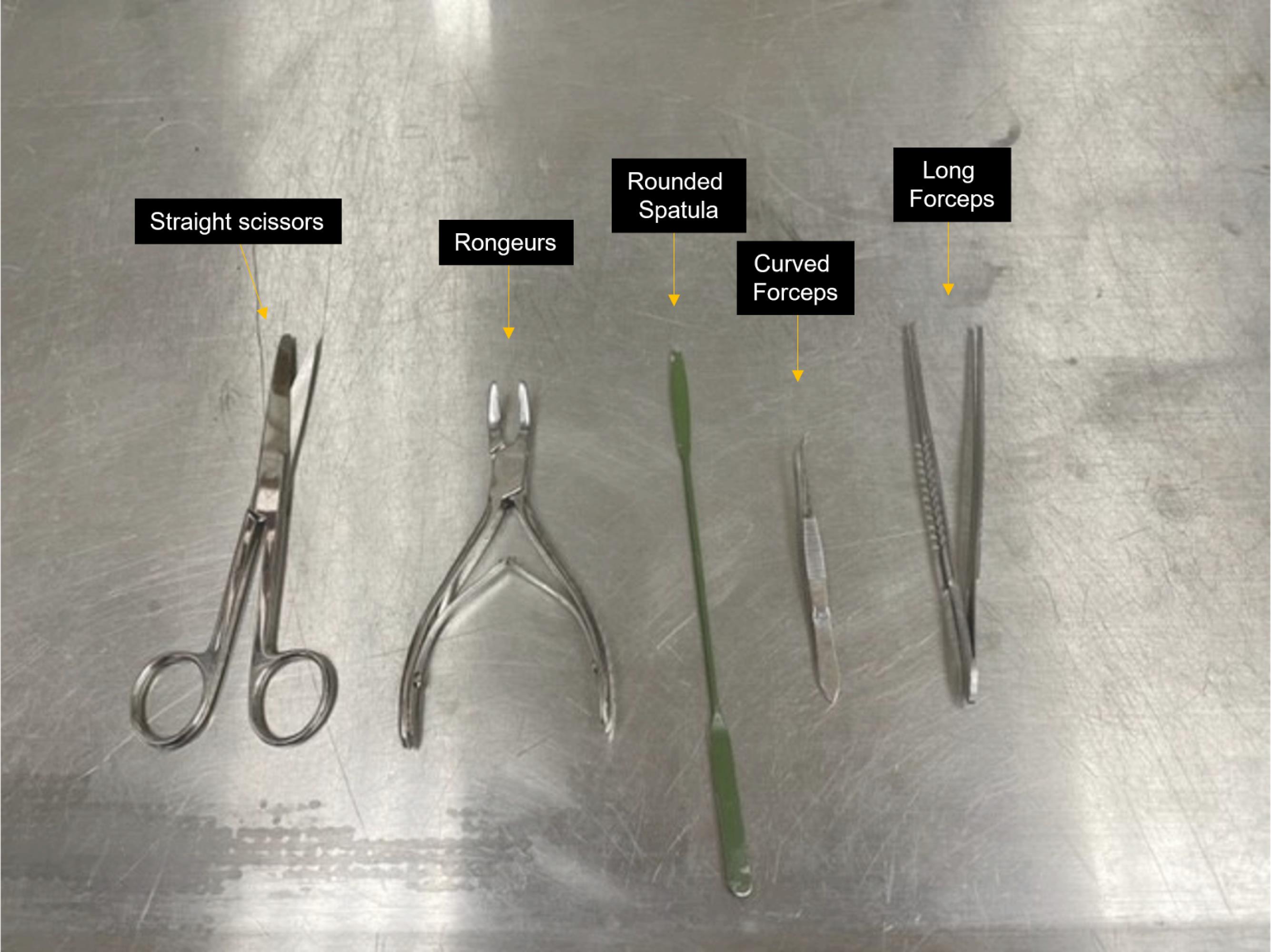
Figure 1. Brain extraction tools. Straight scissors, rongeurs, rounded spatula, and curved and long forceps indicated.

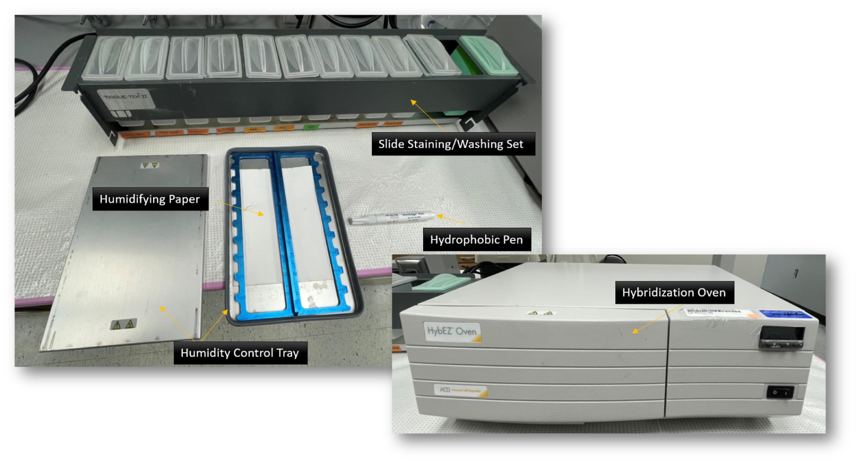
Figure 2. HybEZ II system. Hybridization oven, humidity control tray, humidifying paper, slide staining/washing set (EZ-Batch wash tray and EZ-Batch slide holder), and hydrophobic pen indicated.

Software

1. Zeiss ZEN blue v2.6 or higher for images acquisition and export (https://www.zeiss.com/microscopy/us/products/microscope-software/zen.html#downloads)

2. QuPath 0.3.2 open-source software (https://qupath.github.io/)

3. Microsoft Excel or similar

4. GraphPad Prism 9.4.1 (https://www.graphpad.com/) or similar

Procedure

1. Brain collection (fresh frozen) and storage

   1. In RNase-free conditions (achieved by cleaning the area with RNase AWAY or any other decontaminant such as low concentration bleach), prepare a beaker containing 300 mL of 2-methylbutane, which will sit on dry ice pellets in a stereo foam container under a chemical hood. The temperature of the 2-methylbutane is monitored with an ultralow temperature thermometer. Allow 30–45 min for the 2-methylbutane to reach the temperature of -30 °C, which is optimal to protect the brains from cracking during cryostat slicing and the mRNA from degradation (see Note 1).

   2. Deeply anesthetize the rat with isoflurane (or any other anesthetic) and perform sacrifice by decapitation. Quickly remove the brain from the skull, removing bone and membrane residues that can potentially damage the tissue.

   3. Immediately drop the brain in chilled 2-methylbutane (-30 °C) and snap-freeze for 25 s (see Note 2).

   4. Grab snap-frozen brain with long tweezers and immediately wrap it in aluminum foil. Avoid any thawing of the tissue and immediately store brains on either dry ice or at -80 °C (see Note 3).

   5. Store brains at -80 °C for up to 12 months. It is not recommended to use brains stored for longer periods, as the mRNA degrades progressively.

      
      

   Notes: If researchers intend to fix the brains using formalin, a different protocol including transcardial perfusion must be followed. Brains perfused in formalin should be post-fixed with formalin overnight, transferred to 30% sucrose to cryoprotect the tissue, and snap-frozen in 2-methylbutane for long-term storage.

   1. Cracks in the tissue will make slicing the samples unmanageable for subsequent assay. Freezing the brains in liquid nitrogen (ultralow temperature) will also create cracks, making the tissue unusable.

   2. This time is critical to prevent splitting of the brain’s hemispheres and mRNA degradation. This procedure allows an even and quick freezing of brain tissue and preserves morphology and 100% of the targeted mRNA, especially if the target is low-to-moderately expressed.

   3. Avoid any contact with tools that have not been previously decontaminated.

      
      

2. Preparation of fresh-frozen brain sections

   1. Move brains from -80 °C to -20 °C prior to slicing. Depending on the laboratory conditions, warming the tissue will take a shorter or longer period of time (30 min to a few hours).

   2. Transfer brains from -20 °C to the cryostat’s chamber, whose temperature was previously optimized (-13 °C). Leave brains inside the cryostat for 2–3 h before starting the slicing. The optimal cryostat temperature for brain slicing depends on the device’s model (user manuals typically provide this information). The above equilibration time is sufficient to allow slicing without cracks. If brain is not ready, increase equilibration time. It usually takes longer when the brain is snap-frozen at temperatures lower than -40 or -50 °C.

   3. Decontaminate the external cryostat area in which SuperFrost^® Plus slides will be positioned before mounting. It is recommended to leave slides outside the cryostat to avoid them being too cold and prevent tissue adhesion after slicing (this step very much depends on the environment and cryostat).

   4. Add 2–3 drops of O.C.T. compound in the specimen stage and immediately place the frozen brain at the right orientation and angle to provide an accurate slicing. Make sure the tissue is perpendicular to the stage to avoid uneven sections.

   5. Cut 10 µm coronal slices from the desired region of interest [here, we collected sections containing the substantia nigra (SN)] and immediately mount them by adhesion onto the SuperFrost^® Plus slides. Each slide can contain up to three (depending on the orientation) rat brain sections. Overcrowding the glass slide with tissue sections will obstruct the area necessary to draw the hydrophobic barrier for the subsequent RNAscope assay.

   6. Keep the sections inside the cryostat to dry and store them in an air-tight slide box wrapped with aluminum foil at -80 °C.

   7. Use sectioned tissue within three months. Sectioned tissue is more prone to faster mRNA degradation.

      
      

3. RNAscope assay

   Multiplex assays are performed according to the manufacturer protocols (we outline specific details below). All incubations are performed at 40 °C using a humidity control chamber (HybEZ oven, Advanced Cell Diagnostics). The steps listed below are similar for mRNA target probes and negative controls, unless noted otherwise. It is recommended to run negative controls (one or two sections are sufficient) within each batch of tissue. Target probes were used as follows:

   RNAscope 3-plex negative control probe set (320871): bacterial DapB (in C1, C2, and C3 probe sets)

   RNAscope probe set: Rn-Hcrtr1-C1, Rn-Th-C2, and Rn-Fos-C3. Note that probe channels and fluorophores should be selected considering the expression levels of desired targets. For example, a higher expression gene may be chosen for a wavelength with high autofluorescence in your sample (e.g., 488/green).

   Below, we describe the most representative steps of this procedure. Slides are immersed in slide staining/washing set for each step, unless noted otherwise.

   
   

   1. Fix the sections: remove sections that were previously stored at -80 °C and immediately immerse them in pre-chilled fixative [4% paraformaldehyde (prepared by diluting a 32% stock solution of paraformaldehyde into 1× PBS) at 4 °C] for 40 min. This step must be performed in a fume hood given the toxicity of paraformaldehyde.

   2. Dehydrate the sections: place sections in 50% (1×), 70% (1×), and 100% (2×) ethanol for 5 min each at room temperature.

   3. Create a hydrophobic barrier around each brain section and let it dry for 1 min at room temperature.

   4. Prepare materials necessary to run the assay (wash buffer, target probes, reagents, and hybridization oven).

   5. Pretreat samples by applying protease IV (approximately five drops directly from the bottle; no dilution needed) for 30 min at room temperature inside the humidifying tray and close lid.

   6. Add desired probe to each section and incubate for 2 h at 40 °C inside the humidifying tray (this temperature is the same for all type of probes, including the negative controls). Importantly, apply the negative control probe to one section every time you run an assay.

   7. Hybridize probe(s) using Amp FL-1, -2, -3, and -4 (we used Amp FL-4-Alt A) for 15 or 30 min (see manufacturer’s instructions) at 40 °C. Each amplification step occurs inside the humidifying tray. After each amplification step, the Amp reagents are removed by washing the sections with wash buffer through slide solution wells.

   8. Counterstain using Fluoro-Gel II with DAPI and cover the sections with coverslips. Make sure the sections are almost completely dry before applying the mounting media to avoid creation of bubbles that can prevent target identification and thus quantification.

   9. Store slides in the dark at 4 °C until image evaluation (optimal time is up to one week).

   
   

   Note: It is possible to combine the RNAscope with IHC techniques, allowing the researcher to further clarify cell identity. In this particular combination, only formalin-fixed brain tissue can be used, and IHC will be done as a second step. Advanced Cell Diagnostics provides technical notes for this purpose that can be found here: https://acdbio.com/system/files_force/gated/TN_323100_TechNote_Dual_ISH_IHC_manual_Multiplex_Fluorescent_V2_06222017.pdf.pdf?download=1.

   For pure RNAscope applications that do not require further cellular characterization, it is recommended to use fresh frozen tissue isolations, as explained in this protocol. Advantages include: 1) less supplies needed, which is a cost-saving factor; 2) fewer steps needed to achieve the same result; 3) better tissue quality that potentially translates to high-quality mRNA targeting, which will simplify the quantification process. In formalin-fixed tissue, it is necessary to add a target retrieval step (performed at high temperatures), which can cause tissue damage and prevent a successful probe targeting. Disadvantages of using fresh frozen tissue isolations include an inability to combine IHC assays that require formalin-fixed tissues (see beginning of this note for more details).

   
   

4. Imaging

   1. Turn on scanner and computer.

   2. Start ZEN v2.6 software.

   3. Load slides in tray and insert inside the scanner.

   4. Inspect the slide magazine for accuracy.

   5. Click on wizard to start scan setup.

   6. Select region of interest (ROI)—in this protocol, we analyzed the SN. When selecting ROI, do not include solely the desired section, but expand to include part of the adjacent areas as well.

   7. In brightfield view, inspect contiguous brain areas to make sure you are in the correct ROI.

   8. In the fluorescent view, select desired channels based on the RNAscope assay. We have DAPI (blue), GFP (green), Cy3 (red), and Cy5 (far red).

   9. For particle counts, exposure times were calculated to allow clear detection of small foci in all channels. These are optimal settings for our scanner (see Note 1):

      1. DAPI: 6–8 ms

      2. EGFP: 1,400–1,800 ms

      3. Cy3: 600–800 ms

      4. Cy5: 1,000–1,400 ms

   10. Focus each channel and set parameters for z-stacking.

   11. Z-stacking: RNAscope sections were originally at 10 µm thickness; however, sections lose a few micrometers from the original thickness post processing. We do not need to set up the z-stacking depth to 10 µm, as that depth is not accurate anymore. In order to achieve a valuable number of slices that contain high-resolution transcripts, we set the z-stacking as follows:

       1. Depth: 5.20 µm

       2. Interval between slices: 0.85 µm

       3. Number of slices: 7

   12. Start scan—a few to several hours will be necessary to scan all the sections, depending on the selected ROI.

   13. Save files for subsequent analysis in QuPath (see Note 2).

       
       

   Notes: These are the steps we followed to image our sections using a Zeiss Axioscan Z.1 within the ZEN software environment. Any high-resolution fluorescent or confocal microscope capable of producing z-stack slices can be utilized to achieve similar results. For all analyses, images were captured via 20× objectives that readily enabled identification of discrete foci corresponding to individual transcripts, while retaining sufficient axial resolution to allow all elements of the tissue section to remain well focused. Although we used these specific parameters for capturing a small brain region such as the SN, the same settings can be used for larger regions, obtaining similar results. Limitations of imaging larger regions are related to longer scanning sessions and increased number of focal points to be selected.

   1. It is recommended to not vary settings in a single batch of slides. This will assist in maintaining consistency through the automatic quantification, minimizing variability in the subcellular thresholds, and identifying potential loss of mRNA signal in sections that are older.

   2. The ZEN software automatically saves the scanned images in the .czi format, which includes several types of information, thus creating large files that require specific data management. Most importantly for the next step, CZI files can be opened in QuPath without the need to merge or process the images with other software (especially if ROIs are selected). QuPath will create as many files as the number of scenes scanned in ZEN. If larger ROI is selected and if a unique focal point is missing, it might be necessary to merge the z-stack slices (with maximum projection) to reach the desired focus in each image tile.

      
      

5. RNAscope subcellular quantification using QuPath (user manual: https://qupath.readthedocs.io/en/stable/)

   1. Open QuPath-0.3.2.

   2. Under the Project tab on the left of the screen, click Create project or Open project to retrieve previous projects (Figure 3).

      Notes:

      1. While searching for files, you may have to change file type from “QuPath Files” to “All Files” to access.

      2. If creating a new project, name and save your file, then import images by choosing File -> Project -> Add images -> Choose files -> Import (you may have to expand the window to full screen to see all options).

         
         

      
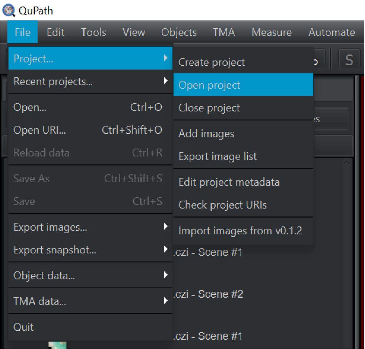
      Figure 3. Screen capture of QuPath. Path to create or open project indicated.

      
      

   3. Double-click the image you want to analyze from the image list.

      1. Under the View tab select Brightness/Contrast . Check the DAPI, EGFP, Cy3, and Cy5 channels (see Figure 4).

      2. Zoom in and out using the scroller on your mouse.

      3. Zoom into an area showing a decent amount of activity from all DAPI, Cy3, and Cy5 channels. Use the adjustable scrolling tool at the top left of the image (z-slice selector) to change the layer of the region you are analyzing. It is imperative to get the clearest image possible to give the most accurate count when analyzing cells and subcellular components.

         
         

      
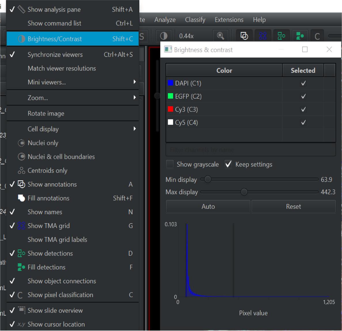
      Figure 4. Screen capture of QuPath. Path to adjust brightness and contrast indicated.

      
      

   4. Once best clarity is achieved, go back to View and Brightness/Contrast and use only the EGFP or Cy5 channels to best view anatomical structures on the slide. Select one of the shapes on the top ribbon and drag to select your ROI (see Figure 5).

      1. Double-click outside of your region to have the outline turn white and the region locked.

      2. You can also use the minimum and maximum display scales to achieve best brightness of your data. It is best to have similar settings across all channels when analyzing images.

         
         

      
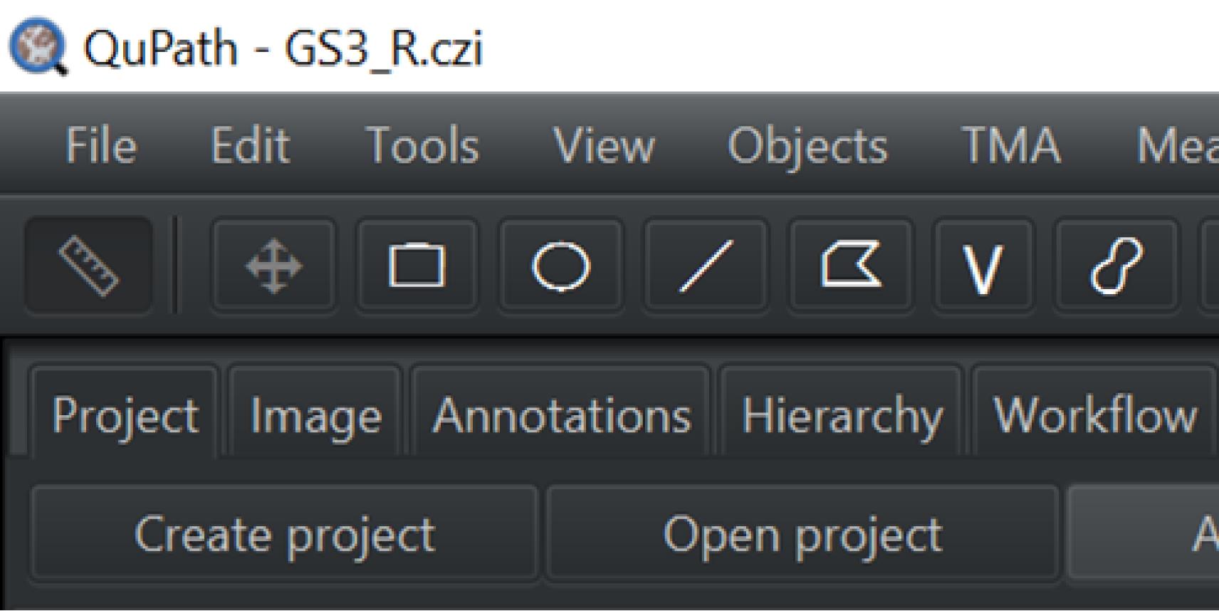
      Figure 5. Screen capture of QuPath. Shapes on the top ribbon are used to outline the ROI.

      
      

   5. Click the Analyze tab, then Cell Detection and Cell Detection again (see Figure 6).

      Change parameters to match the list below and then click Run .

      1. Background radius: 10 µm (if background subtraction is considered, 0 means no background subtraction).

      2. Median filter radius: 2.0 µm (reduce image texture/smooth intensity vibrations).

      3. Sigma: 2.0 µm [control/reduce the noise effect; with a smaller number you will get more nucleus (more fragments)].

      4. Maximum area: 300 µm² (define the range of nucleus size).

      5. Threshold: 30 (intensity parameter for nucleus objects).

         
         

      
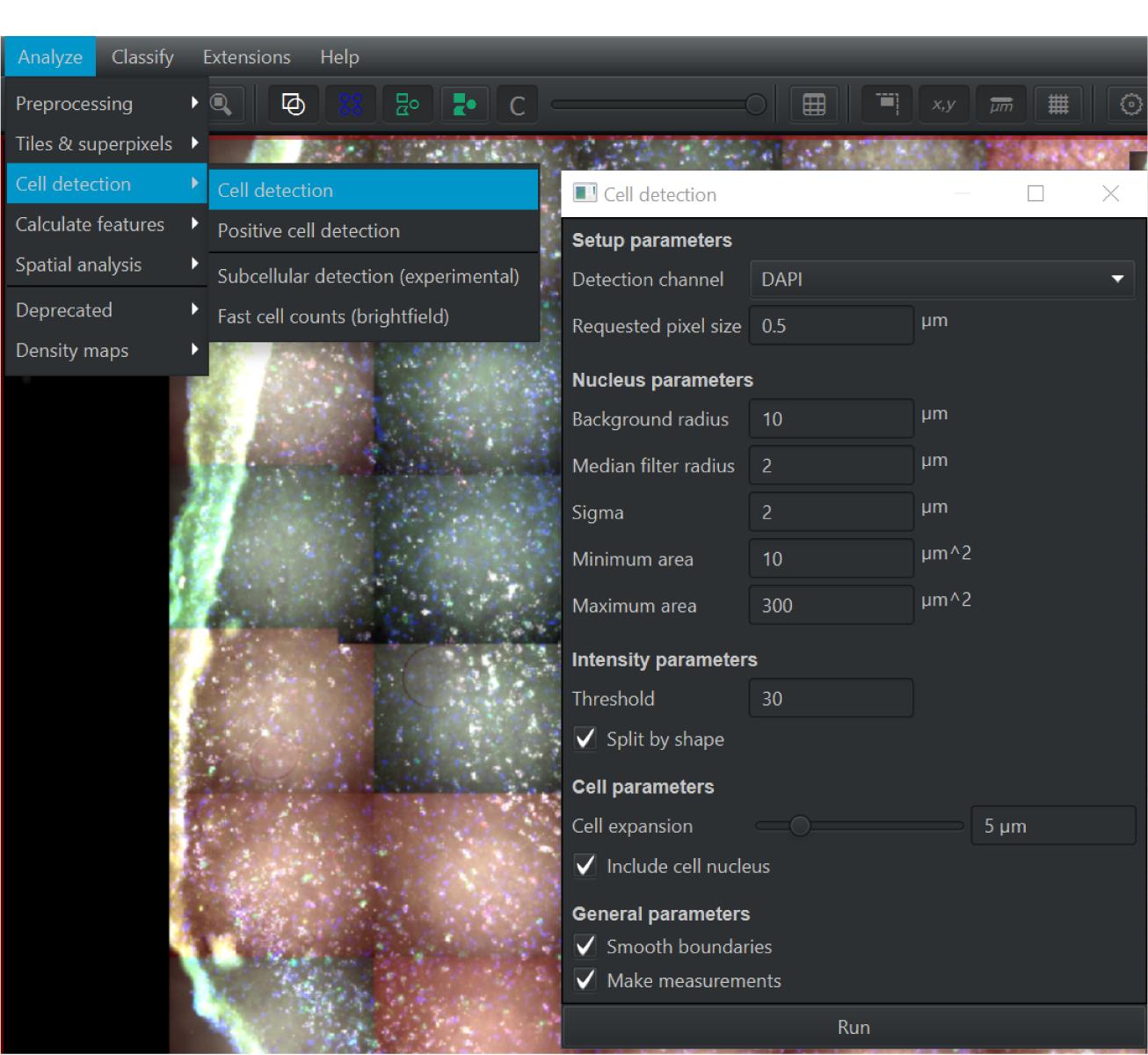
      Figure 6. Screen capture of QuPath. Parameters used for cellular detection are indicated.

      
      

   6. After analyzing for Cell Detection , you will need to zoom in and inspect the quality of the segmentation. Some cells may have been grouped together and only counted as one, and other cells may have been segmented to count as multiple cells (see Figure 7). You can alter the median filter radius, sigma, and threshold and re-run the cell detection until best segmentation is achieved (see Figure 8).

      Poor segmentation can indicate that you need to alter the parameters of your run, or that you need to achieve better clarity of your ROI.

      
      

      
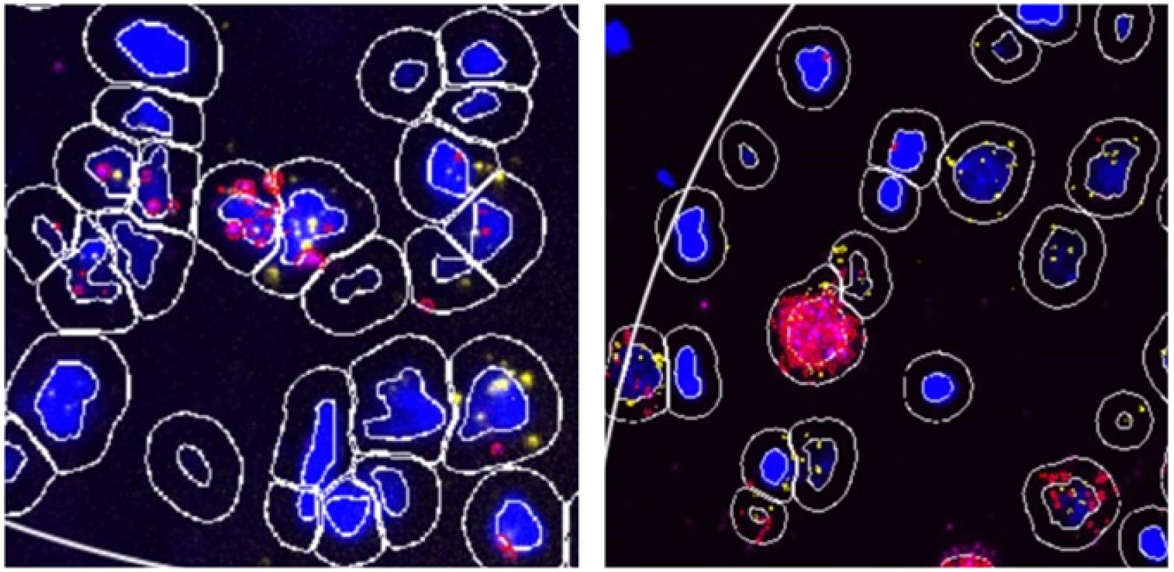
      Figure 7. Representative QuPath image with poor (left) and good (right) nuclear segmentation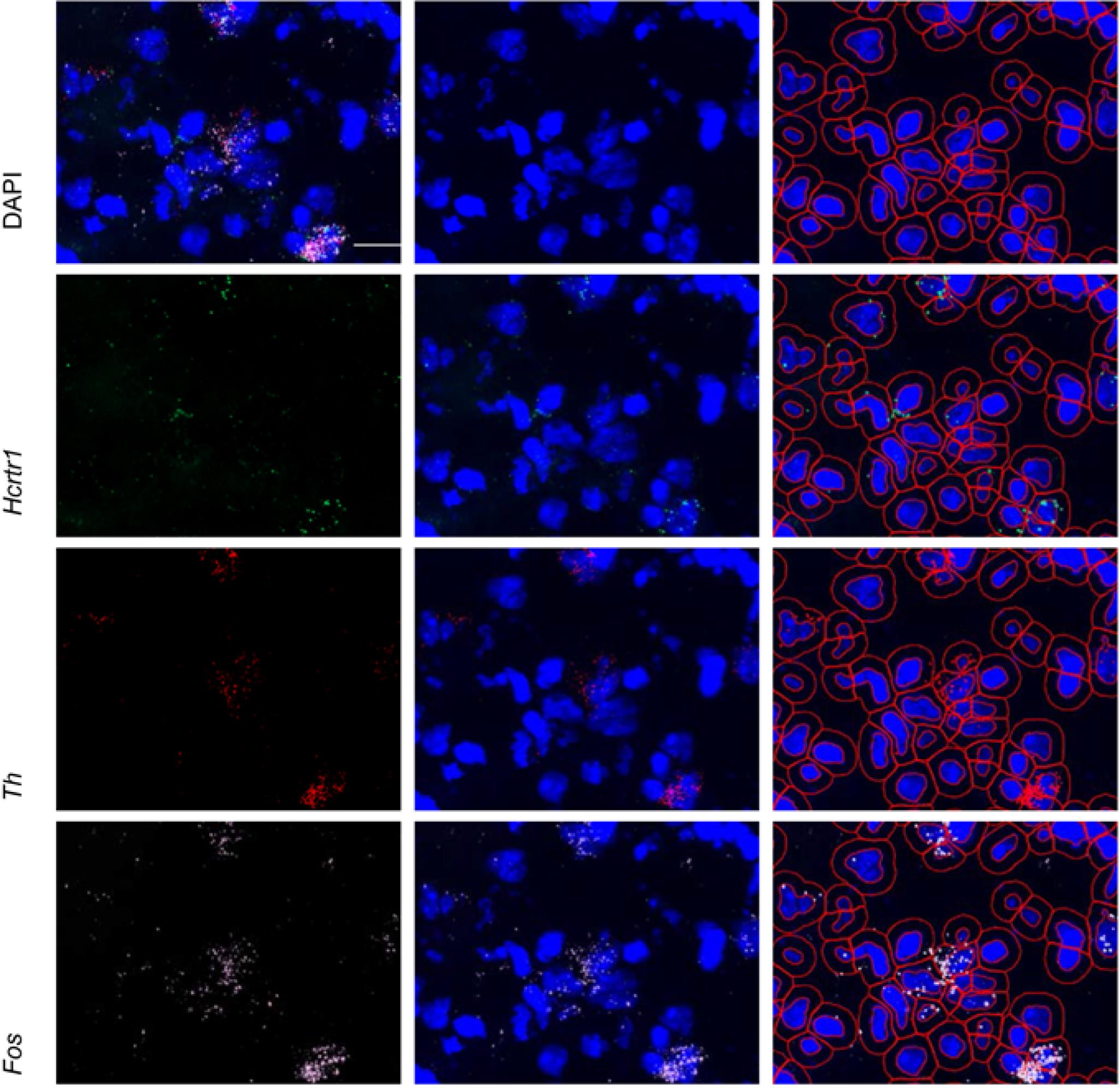

      
      

      
      Figure 8. Representative probe expression and nuclear/subcellular segmentation in QuPath. Top left panel shows representative expression of DAPI (blue), Hcrtr1 (green), Th (red), and Fos (white) in the substantia nigra. Individual probe expression shown alone (left) or with DAPI (middle). Right panel shows the cellular and sub-cellular identification through QuPath for each channel. Scale bar = 20 µm.

      
      

   7. Click Analyze , then Cell Detection , and then Subcellular Detection (see Figure 9). Parameters should be set as below; then, click Run .

      Note: Threshold for DAPI should be set to 0; other thresholds shown here depend on the dot’s intensity for each channel.

      1. Channel 2 threshold: 600

      2. Channel 3 threshold: 600

      3. Channel 4 threshold: 600

      4. Check all three boxes that say “smooth before detection,” “split by intensity,” and “split by shape.”

      5. Expected spot size: 0.5 µm²

      6. Min spot size: 0.5 µm²

      7. Max spot size: 15 µm²

         
         

      
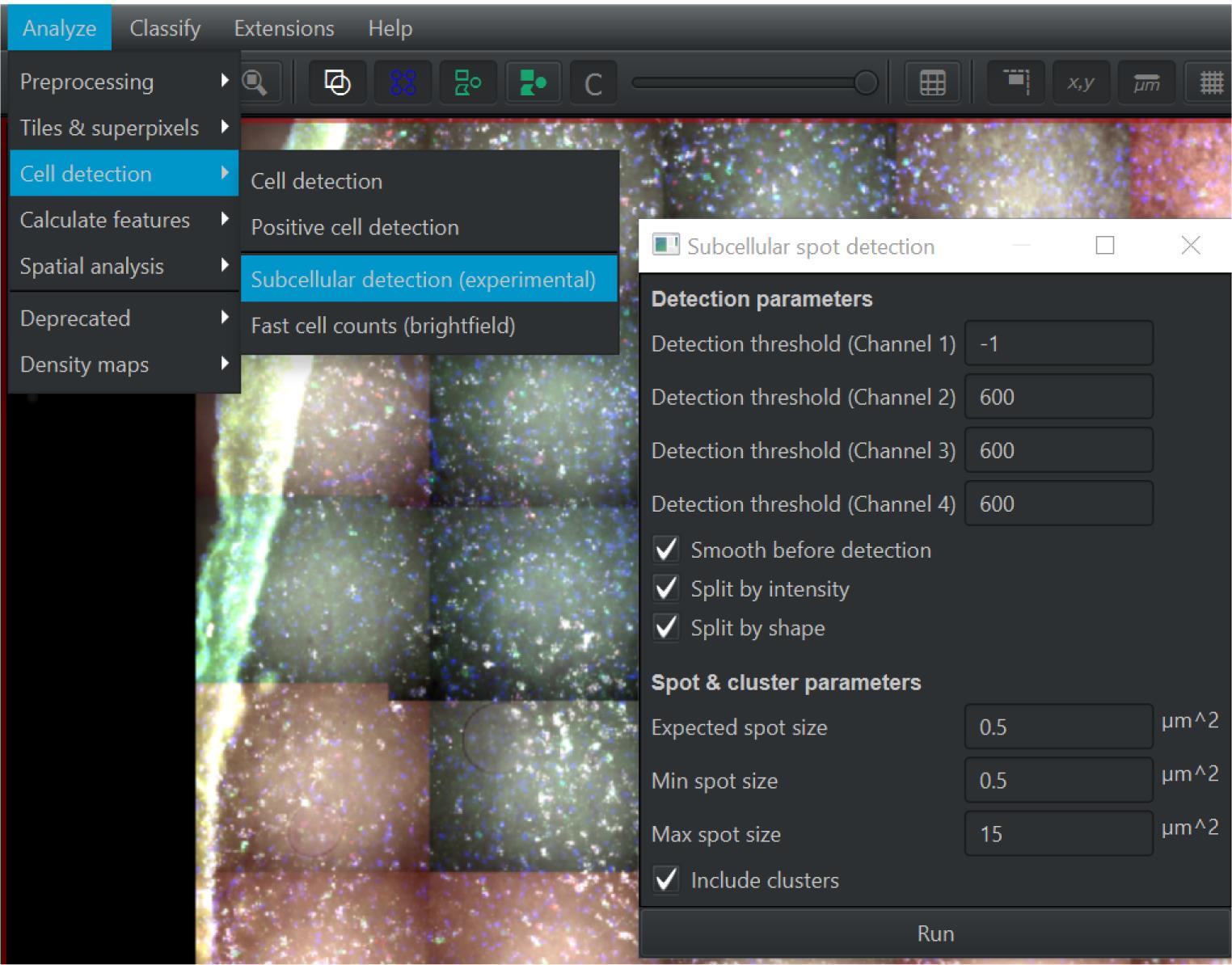
      Figure 9. Screen capture of QuPath. Parameters used for subcellular detection are indicated.

      
      

   8. After analyzing for subcellular detection, inspect again for quality and accuracy of data collection. Alter parameters of maximum spot size and threshold to increase quality (see Figure 9).

      You can return to View and Brightness/Contrast and double-click on a channel to change its color, as sometimes the subcellular components and the circle identifying them after analysis are the same color.

   9. Once best quality of data is collected, go to Measure and Show Detection Measurements (see Figure 10). Choose Copy to Clipboard and open Excel to paste all the data.

      The only other piece of data to collect from inside QuPath is the number of cells. You can access this by clicking Annotations on the left side of the screen; at the top-left you will see Annotation (Ellipse) (e.g., 1006/3650 objects) . The first of the two numbers is the number of cells identified in QuPath. You can double-check this by viewing how many nuclei area you have in the Excel data

      
      

      
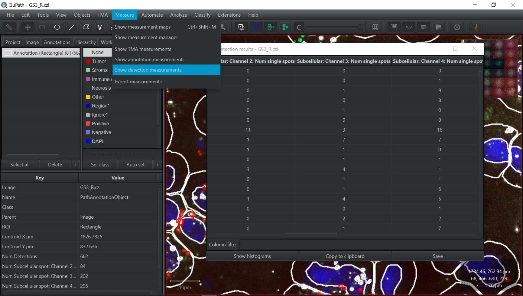
      Figure 10. Screen capture of QuPath. Pathway to detection measurements indicated.

      
      

   10. In Excel (Figure 11), the only columns you need to keep for data collection are:

       1. Nucleus: Area

       2. Subcellular channel 2: Number of single spots

       3. Subcellular channel 3: Number of single spots

       4. Subcellular channel 4: Number of single spots

   11. Find average nucleus area by selecting the letter of the column in which the nuclei area is listed; under Sort and Filter select Sort Smallest to Largest . Insert the average function in an empty cell, select all the cells containing nucleus areas, and then click enter.

   12. Again, sort smallest to largest on the subcellular channel 2 column and count the number of single spots above your set threshold, including the threshold (i.e., if my threshold is 5, count all the subcellular single spots showing 5 or more spots).

       Repeat for subcellular channels 3 and 4.

       
       

   
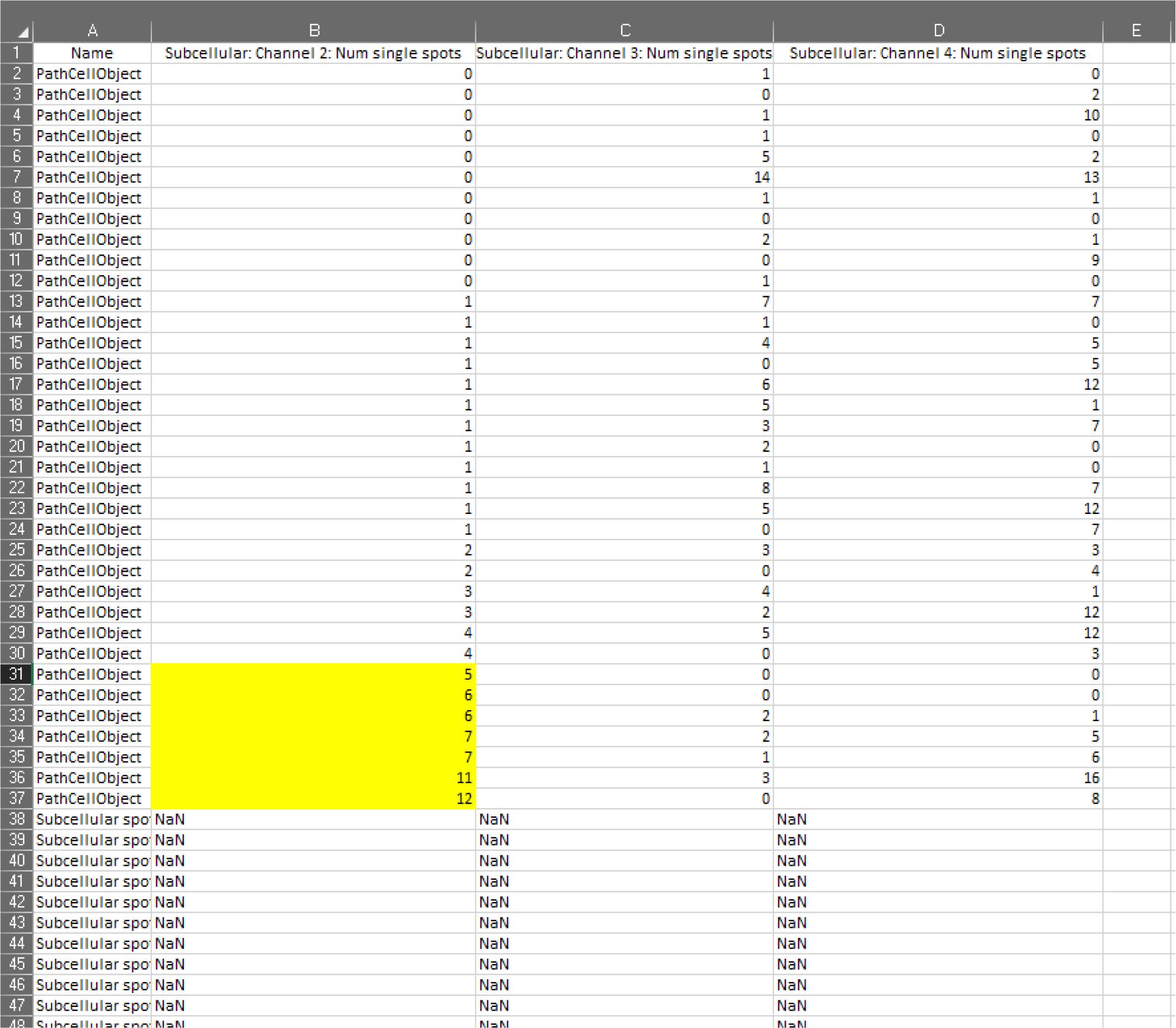
   Figure 11. Screen capture of Excel. Subcellular detections are sorted for channel 2, and those cells above the threshold are highlighted in yellow.

   
   

   Once all the above parameters have been optimized, it is possible to expedite the analysis workflow using customized automatisms (see Figure 12). We can create scripts deriving from the steps shown above or create customized scripts, if additional parameters or extensions will be used (e.g., Stardist—deep learning models). For simplicity, we describe the steps to generate an automatism from an existing workflow.

   1. Go to Automate -> Show Workflow Command History -> Select desired steps -> Create script -> Save script.

   2. Open generated script and inspect all the lines for accuracy. Modify channel and analysis parameters according to optimized workflow. Save script and run it for any other selected ROI.

      Automated analysis saves minutes of work allowing to complete tasks in fractions of time.

   
   

   
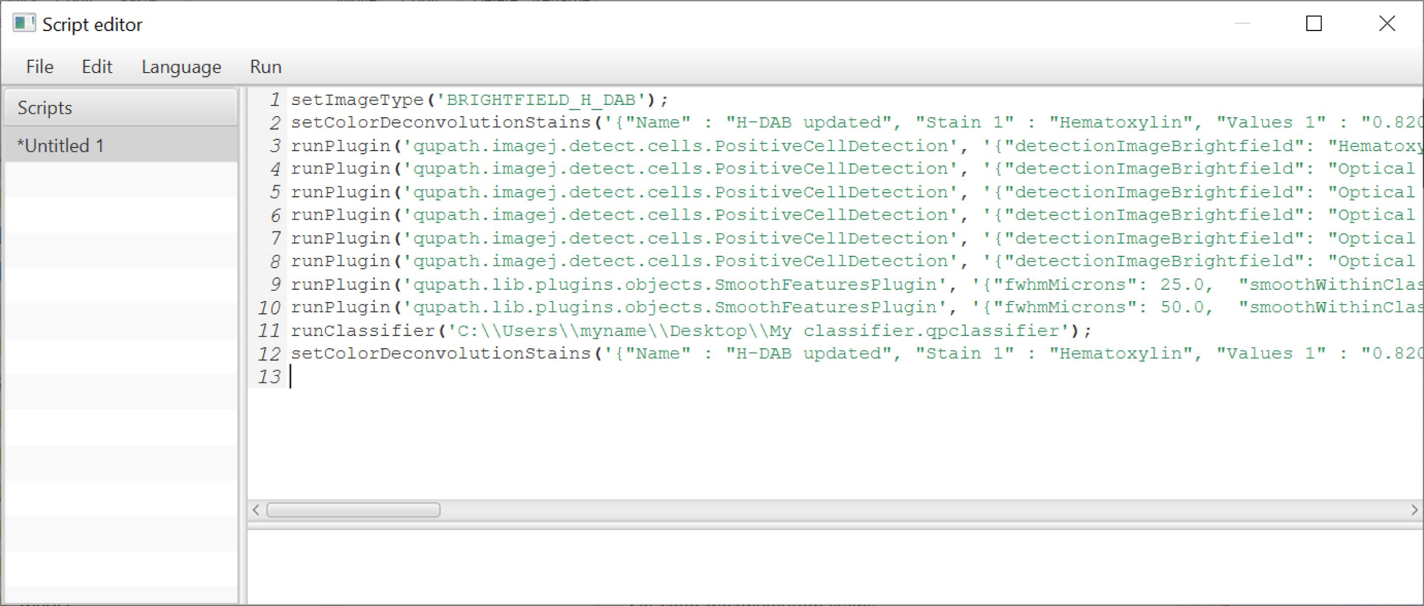
   Figure 12. Example of script used in QuPath to run automated analysis

Data analysis

Each time you run an RNAscope assay it is critical to determine an analysis threshold, which will serve as the criteria for inclusion or exclusion of data in processed images. Punctate expression should be quantified in each channel of negative control probe-processed tissue, as described above (see Figure 13 for representative images). Calculate the average and standard deviation of puncta in each channel. The sum of these values is your threshold for all processed images.

Note: Some cells will have zero puncta in a given channel; when calculating the average punctate expression in negative control probe-processed images, be sure to only include values >0; inclusion of 0 values will artificially lower your threshold and influence your data (see example in Table 1 and Figure 14). The threshold will be unique for each channel (e.g., Table 1).

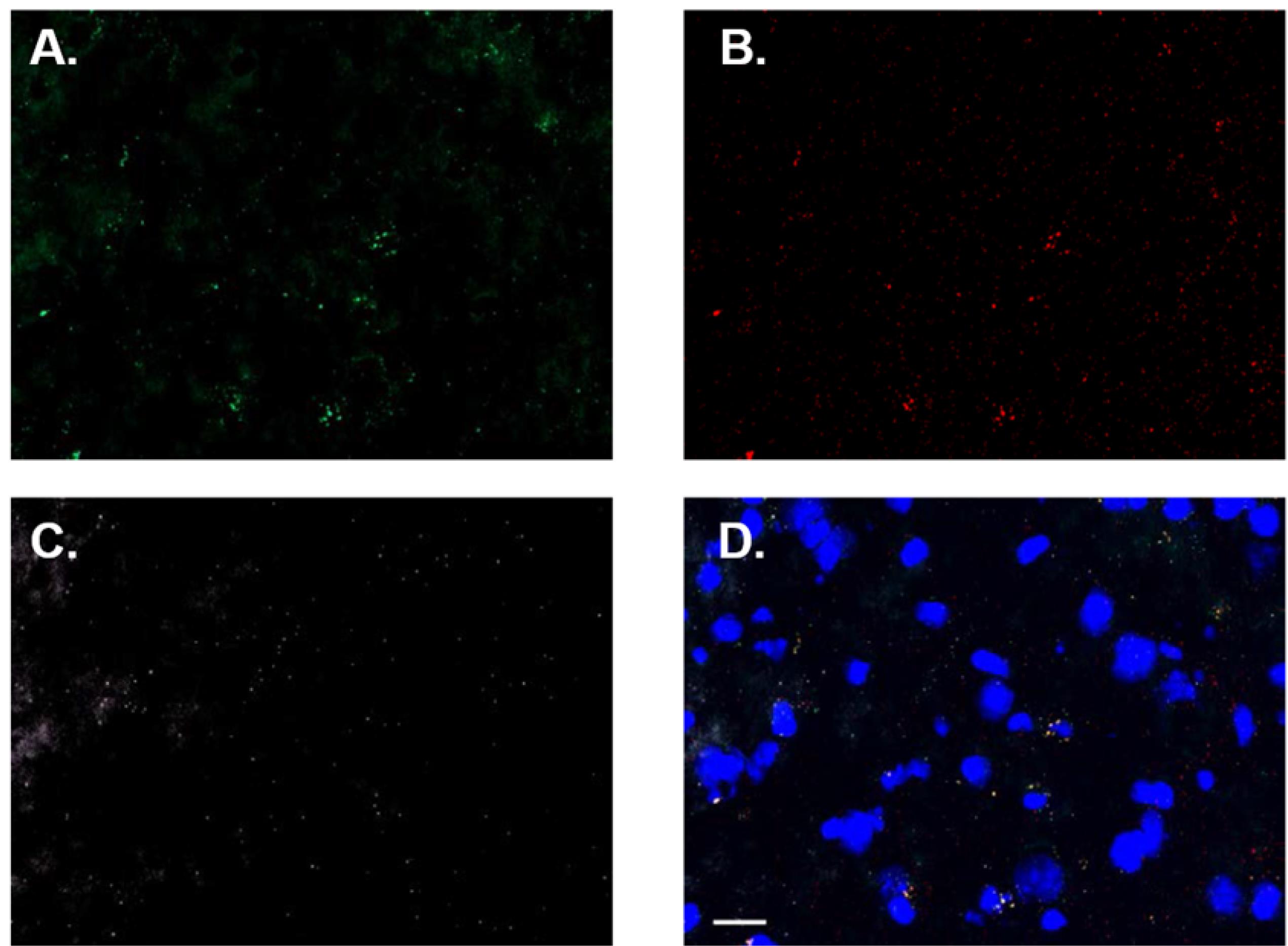
Figure 13. Representative negative control probe-processed tissue images. Non-specific signal in green–POLR2A (A), red–PPIB (B), white–UBC (C), and merged (D) channels shown. Images shown with increased brightness due to low fluorescent signal. Scale bar = 20 µm.

Table 1. Example threshold calculations for each channel from negative control probe-processed tissue images. Threshold is determined by adding the average and standard deviation of the number of puncta per channel. Including zero values artificially lowers this threshold.

	Channel 2 (green)	Channel 3 (red)	Channel 4 (far red)
Average number of puncta (including zero values)	0.76	1.90	0.43
Standard deviation	1.48	2.92	1.16
Threshold (including zero values)	2.24	4.82	1.59
Average number of puncta (excluding zero values)	2.17	3.43	2.10
Standard deviation	1.48	2.91	1.16
Threshold (excluding zero values)	3.65	6.34	3.26

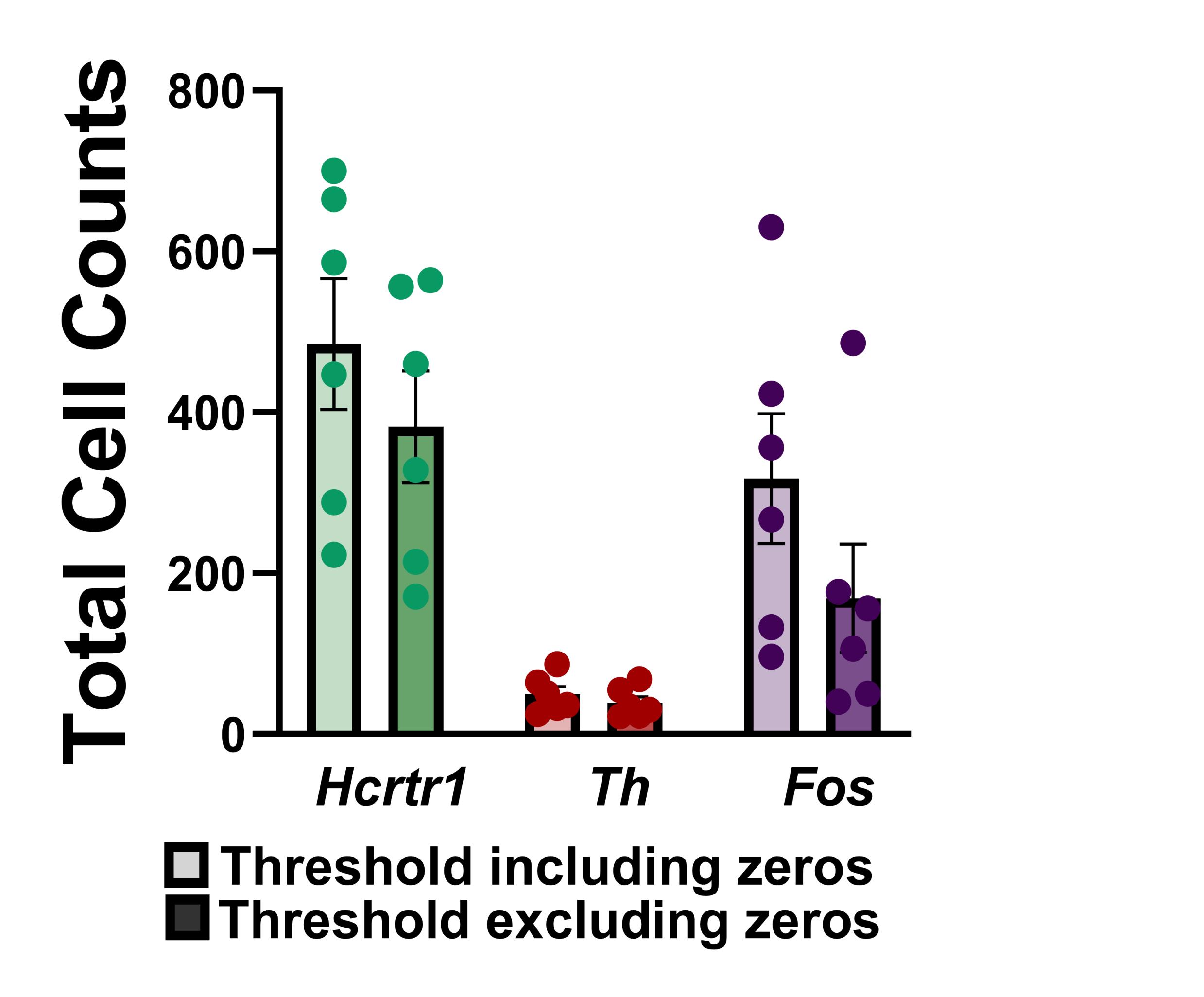
Figure 14. Influence of threshold on cell counts using RNAscope-processed tissue.

Figure shows the total number of neurons determined to be positive for expression of Hcrtr1 (green bars), Th (red bars), or Fos (purple bars) in regions analyzed within the substantia nigra from six rats. Using a lower threshold calculated by inclusion of zero values in the negative control probe-processed images (see Data Analysis section) results in a higher number of positive cell counts (lighter bars), compared to the use of a more stringent threshold value calculated by averaging punctate expression only in cells with ≥ 1 puncta (darker bars).

Acknowledgments

This protocol was adapted from Avegno et al. Addiction Biology (2021, DOI: 10.1111/adb.12990). The work described here was supported by the National Institute of Health (U01AA028709, R01AA023305 to NWG and K01AA028541 to EMA) and United States Department of Veterans Affairs, Biomedical Laboratory Research and Development Service (Merit Award I01 BX003451 to NWG).

Competing interests

Nicholas W. Gilpin owns shares in Glauser Life Sciences, a company with interest in developing therapeutics for mental health disorders. There is no direct link between those interests and the work contained herein. All other authors report no conflicts of interest.

Ethics

All procedures were approved by the Institutional Animal Care and Use Committee of the Louisiana State University Health Sciences Center and were in accordance with the National Institutes of Health guide for the care and use of Laboratory animals (NIH Publications No. 8023, revised 1978).

References

1. Avegno, E. M., Kasten, C. R., Snyder, W. B., 3rd, Kelley, L. K., Lobell, T. D., Templeton, T. J., Constans, M., Wills, T. A., Middleton, J. W. and Gilpin, N. W. (2021). Alcohol dependence activates ventral tegmental area projections to central amygdala in male mice and rats. Addict Biol 26(4): e12990.
2. Bankhead, P., Loughrey, M. B., Fernandez, J. A., Dombrowski, Y., McArt, D. G., Dunne, P. D., McQuaid, S., Gray, R. T., Murray, L. J., Coleman, H. G., et al. (2017). QuPath: Open source software for digital pathology image analysis. Sci Rep 7(1): 16878.