- Protocols

- Articles and Issues
- For Authors
- About
- Become a Reviewer

Proteome Integral Solubility Alteration (PISA) Assay in Mammalian Cells for Deep, High-Confidence, and High-Throughput Target Deconvolution
Published: Vol 12, Iss 22, Nov 20, 2022 DOI: 10.21769/BioProtoc.4556 Views: 4488
Reviewed by: Chiara AmbrogioAnna A. ZorinaAnonymous reviewer(s)
Original research article
The authors used this protocol in:

Feb 2022
Advertisement


Protocol Collections
Comprehensive collections of detailed, peer-reviewed protocols focusing on specific topics


Related protocols
Abstract
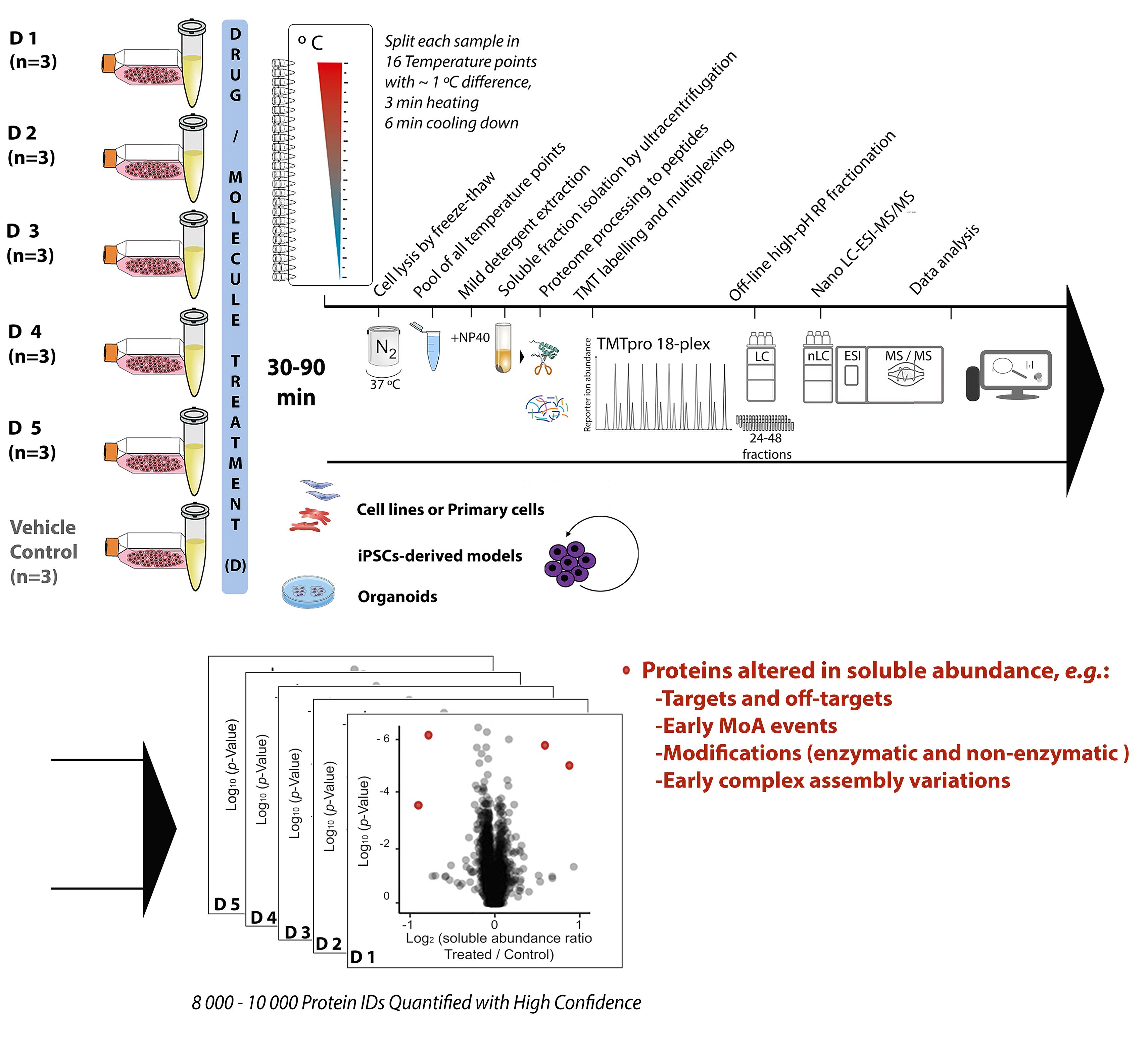
Chemical proteomics focuses on the drug–target–phenotype relationship for target deconvolution and elucidation of the mechanism of action—key and bottleneck in drug development and repurposing. Majorly due to the limits of using chemically modified ligands in affinity-based methods, new, unbiased, proteome-wide, and MS-based chemical proteomics approaches have been developed to perform drug target deconvolution, using full proteome profiling and no chemical modification of the studied ligand. Of note among them, thermal proteome profiling (TPP) aims to identify the target(s) by measuring the difference in melting temperatures between each identified protein in drug-treated versus vehicle-treated samples, with the thermodynamic interpretation of “protein melting” and curve fitting of all quantified proteins, at all temperatures, in each biological replicate. Including TPP, all the other chemical proteomics approaches often fail to provide target deconvolution with sufficient proteome depth, statistical power, throughput, and sustainability, which could hardly fulfill the final purpose of drug development. The proteome integral solubility alteration (PISA) assay provides no thermodynamic interpretation, but a throughput 10–100-fold compared to the other proteomics methods, high sustainability, much lower time of analysis and sample amount requirements, high confidence in results, maximal proteome coverage (~10,000 protein IDs), and up to five drugs / test molecules in one assay, with at least biological triplicates of each treatment. Each drug-treated or vehicle-treated sample is split into many fractions and exposed to a gradient of heat as solubility perturbing agent before being recomposed into one sample; each soluble fraction is isolated, then deep and quantitative proteomics is applied across all samples. The proteins interacting with the tested molecules (targets and off-targets), the activated mechanistic factors, or proteins modified during the treatment show reproducible changes in their soluble amount compared to vehicle-treated controls. As of today, the maximal multiplexing capability is 18 biological samples per PISA assay, which enables statistical robustness and flexible experimental design accommodation for fuller target deconvolution, including integration of orthogonal chemical proteomics methods in one PISA assay. Living cells for studying target engagement in vivo or, alternatively, protein extracts to identify in vitro ligand-interacting proteins can be studied, and the minimal need in sample amount unlocks target deconvolution using primary cells and their derived cultures.
Graphical abstract:
Background
Correct target identification and elucidation of the fine mechanism of action (MoA) of ligands, both covalent and noncovalent, representing research-grade as well as already approved drugs, are both key and major bottlenecks in drug development and drug repurposing (Swinney and Anthony, 2011).
The case of cancer drugs is a clear example of this. It is estimated that 97% of the tested anticancer molecules never make it to the clinic, often because the proposed mechanism of action is incorrect and the observed drug effects are due to off-target toxicity (Lin et al., 2019).
Moreover, the high rate of clinical trial failures clearly indicates the need to seek more precise information on drug targets and the MoA more strictly related to the drug. Therefore, all methodological efforts in this direction are very relevant and worth pursuing. Among the -omics sciences, genomics and transcriptomics have been applied in drug development because of limited operational cost for comparing normal and diseased states, measuring changes in transcription levels, pharmacogenomics, and stratifying patients in clinical trials. However, only mass spectrometry (MS)-based proteomics—and particularly chemical proteomics—can fill in the gap in knowledge of the drug–target–phenotype relationship, by exploring it at a proteome-wide level, with deep proteome coverage, and unbiasedly. Chemical proteomics encompasses different methods, each attacking the problem from a different angle, and each limited by the original intention and experimental design.
The MS-based approaches for the identification of protein interactions using affinity-based purification with chemically engineered ligand probes (Rix and Superti-Furga, 2009) have the strong limitation of the uncertainty in the functional properties of the engineered bait compared to the original ligand. Moreover, even with a well-performing click chemistry used to lock the protein to the bait, the always present promiscuity in binding results in locking background proteins. Additionally, the non-specific noncovalent interactions in the affinity enrichment step lead to an increased background (Wright and Sieber, 2016). The consequent limited specificity of the results called for the development of target deconvolution approaches requiring no chemical modification of the ligand. Therefore, the use of unbiased, proteome-wide, and MS-based proteomics approaches for target deconvolution (Kwon and Karuso, 2018) have recently gained a major place in chemical proteomics.
A promising proteome-wide approach for protein target identification in living cells uses the specificity of protein abundance regulation in ligand-induced late apoptosis (Gaetani and Zubarev, 2019). The concept, originally developed for chemotherapeutics, was also successfully applied to metallodrugs and nanoparticles (Chernobrovkin et al., 2015; Lee et al., 2017; Tarasova et al., 2017), and then extended to a vast library of cancer drugs and multiple cell lines (Saei et al., 2019). This last work produced an online tool assisting in the deconvolution of targets for molecules exhibiting significant cell toxicity at 48h, showing specific regulation of drug targets and mechanistic factors in late apoptosis. However, limitations regarding elucidation of direct primary drug targets and mechanisms direct to the general call for orthogonal methods based on alternative principles.
In thermal proteome profiling (TPP) (Savitski et al., 2014; Franken et al., 2015), drug targets are identified by the increase in protein melting temperatures (Tm) obtained by curve fitting of all temperature points measured in the tandem mass tag (TMT) batch used for each of the drug- or vehicle-treated biological replicates (2 h treatment). Each biological replicate requires a complete TMT batch, and the overall TPP experiment requires as many TMT batches as the biological samples. Therefore, in TPP, scalability and the use of more than two biological replicates per treatment type is complicated by the high sample amounts and costs; straightforward interpretation of the curves obtained within complex intracellular environment as “protein melting” is questionable; data analysis of multibatch TMT and suboptimal curve fitting damage the depth of proteome coverage, with increasing missing values among replicates resulting in false positive and false negative rates (Brenes et al., 2019).
The proteome integral solubility alteration (PISA) assay, commonly named “PISA,” in which this protocol focuses, provides deep and quantitative proteome analysis of the changes in amount of the soluble fraction of each identified protein. Each drug-treated or vehicle-treated sample—thus, each soluble proteome—is first exposed to a gradient of heat as solubility perturbing agent, inducing protein aggregation (Gaetani et al., 2019). Each soluble fraction is isolated, and then deep and quantitative proteomics is applied across all multiplexed biological samples. PISA was proven correct in finding primary and secondary targets in its proof-of-principle work using different drugs with known targets in different cell lines and respective lysates. The method successfully performed target identification and provided elements for MoA elucidation by comparing parallel experiments in living cells and lysates. Indeed, PISA can be applied to living cells for studying target engagement in vivo, or alternatively to protein extracts to identify in vitro ligand-interacting proteins. Further studies applying PISA on an antimicrobial molecule showing anticancer properties were recently published, proving PISA correct also in cases where the target is not known, as it was further validated with follow-up experiments of a different nature (Heppler et al., 2022). Using a statistically relevant number of biological replicates for each tested condition within the same TMT batch, PISA is designed to gain the full robustness and quantification accuracy of TMT multiplexing, and to provide high throughput and high sustainability to target deconvolution, with depth of proteome analysis up to approximately 10,000 proteins in human cells (using current protocols). With up to 18 biological samples per TMT-multiplexed assay, and no thermodynamic interpretation, the PISA assay maximizes throughput, sustainability, proteome coverage, statistical power of analysis (three or more replicates), confidence in results, and several drug molecules analyzed per TMT batch (up to five). The PISA assay conveniently takes advantage of the latest TMTpro technology (Thermo Scientific) (Li et al., 2020b), further extended to 18-plex, allowing for up to nine biological replicates of the ligand compared to vehicle in a single LC–MS/MS experiment. Further developments in TMT technology will immediately increase the PISA throughput. The PISA assay also integrates the advances in deep, quantitative proteomics, including extensive off-line high pH fractionation and nanoscale liquid chromatography (nLC)–MS of all produced fractions.
PISA does away with the sigmoidal solubility-temperature curves and Tm derivation, as each sample is split in equal portions that are exposed to different temperatures before being recomposed into one and multiplexed with the other samples. In PISA, the final amount of each protein would correspond to the integral of a putative solubility-temperature dependence curve, regardless of its shape and function. The information lost on the shape of the solubility-temperature dependence curves turned out to be largely irrelevant for drug target identification. The normalized difference between drug- and vehicle-treated samples is called ΔSm; the ratio (R) of the soluble abundances is also used, and sometimes more advantageous for final data analysis. The number of samples analyzed in PISA by MS is the same regardless of the number of temperature points used, while in TPP, these numbers are in a linear dependence. Therefore, PISA can easily afford a larger number of temperature points, increasing precision of comparative quantification across replicates, which is already increased by removal of the curve fitting. Furthermore, to increase the ΔSm (or R) sensed in PISA by specific targets at a specific temperature range, the last can be narrowed around the region with the highest solubility changes, for most proteins of interest (Li et al., 2020a).
The original PISA assay makes use of the temperature to challenge protein solubility, as temperature is the most optimized and standardized protein aggregation/precipitation agent, easy to control, and removable from samples; however, different PISA assays using organic solvents (Van Vranken et al., 2021) or kosmotropic salts (Beusch et al., 2022) have also been developed. These temperature-free variants of the PISA assay prove its correct design, to robustly interpret and reproducibly measure the proteome amount changes in the soluble fraction as protein solubility rather than protein melting variations.
All in all, PISA increases the throughput by 10–100-fold compared to any other chemical proteomics method, routinely allowing experiments with three or four biological replicates for several compounds simultaneously, and making possible larger studies that would otherwise be prohibitively expensive. Of further relevance, PISA also enables analysis of much reduced sample amounts, and is currently optimized for minimal cell amounts typical for cell culture models of primary cells, iPSC-derived cell cultures, and 3D cell cultures, including organoids.
PISA can also be applied to a range of ligand concentrations, with preferential selection of the target binding at a lower concentration (2D PISA) (Gaetani et al., 2019). In PISA, the reproducible protein amount changes between the soluble fractions of the drug-treated samples and controls can represent the target and off-target interactions, factors involved in early MoA, modified proteins, and early complex assembly variations occurred during the applied drug treatment. The major PISA capabilities of target deconvolution and MoA elucidation reside in the versatility to accommodate within the same TMT multiplex a project design tailored for specific needs, for example, with robust comparisons among various compounds, or incubation at various time points, drug concentrations, or cells. For fuller target deconvolution, PISA can also be integrated in one multiplex with its orthogonal method expression proteomics—altogether named PISA-Express. In PISA-Express, both the proteome regulation as cellular adaptation / response to the drug in 24 h/48 h, together with the solubility shift for 30–90 min incubation in PISA are studied. A relevant feature of PISA-Express is the possibility to analyze solubility alteration at longer times of drug incubation, when cellular protein expression is altered by the drug treatment, and the solubility shifts can be normalized to the total protein abundance variation, due to the integration of PISA and expression proteomics in the same analysis (Sabatier et al., 2021). A third analysis dimension—RedOx proteomics—can also be integrated, and allows the 3D PISA profiling into a single TMT multiplex set, which could be a future industrial standard analysis for drug target identification and MoA elucidation.
Materials and Reagents
Cell culture
Tubes for centrifugation 50 mL and 15 mL (Sarstedt, catalog numbers: 62.559 and 62.554.502)
Sterile 25 cm2 cell culture flask (Sarstedt, catalog number: 83.3910.002)
Cell culture medium [e.g., Dulbecco’s modified Eagle’s medium (DMEM)] (Thermo Fisher Scientific, catalog number: 11685260; original manufacture: Lonza, catalog number: BE12-614F)
Fetal Bovine Serum (FBS, Thermo Fisher Scientific, catalog number: 11560636)
Penicillin-streptomycin solution (Gibco, catalog number: 15140-122)
L-Glutamine (Gibco, catalog number: A2916801)
Ca2+Mg2+-free Dulbecco’s PBS (Cytiva, catalog number: 10462372)
TrypLE express enzyme solution (Thermo Fisher Scientific, catalog number: 12605036)
Dimethyl sulfoxide solution (DMSO, Merck, catalog number: D8418)
PISA treatment
0.2 mL PCR tube strips with caps (Thermo Fisher Scientific, catalog number: AB0452)
Protein low-binding tubes for centrifugation, 1.5 mL and 2 mL (Thermo Fisher Scientific, catalog numbers: 10708704 and 10718894; original manufacture: Eppendorf, catalog number: 0030108116 and 0030108132)
1.5 mL polypropylene tubes for ultracentrifugation (Beckman Coulter, catalog number: 357448)
Ca2+Mg2+-free Dulbecco’s PBS (Cytiva, catalog number: 10462372)
100× protease inhibitor cocktail solution (Thermo Fisher Scientific, catalog number: 78439)
Liquid N2 in a container
Nonidet P-40 (NP40) (Thermo Fisher Scientific, catalog number: 11596671)
Milli-Q water
Cell lysis buffer (see Recipes)
20% NP40 (see Recipes)
Soluble protein fraction processing
Micro-BCA assay kit (Thermo Fisher Scientific, catalog number: 23235)
Dithiothreitol (DTT, Merck, catalog number: D0632)
Iodoacetamide (IAA, Merck, catalog number: I6125)
Acetone (Thermo Fisher Scientific, catalog number: 10417440)
4-(2-hydroxyethyl)-1-piperazinepropanesulfonic acid (EPPS, Merck, catalog number: E9502)
Urea (Merck, catalog number: U5378)
Lyophilized LysC enzyme (FUJIFILM Wako Pure Chemical Corporation, catalog number: 125-05061)
Lyophilized sequencing grade modified trypsin enzyme (Promega, catalog number: V5111)
Trypsin Resuspension Buffer (Promega, catalog number: V5111)
Tandem Mass Tag (TMT) 10-plex, TMTproTM 16-plex, or TMTproTM 18-plex isobaric label reagent set (Thermo Fisher Scientific, catalog numbers: 90110, A44520, or A52045)
Water-free acetonitrile (Thermo Fisher Scientific, catalog number: 10222052)
50% hydroxylamine solution (Thermo Fisher Scientific, catalog number: 90115)
Trifluoroacetic acid (TFA, Merck, catalog number: 302031)
Methanol (Skandinaviska Genetec, catalog number: RH1019/2.5)
Acetonitrile (ACN, Thermo Fisher Scientific, catalog number: A955-212)
Formic acid (FA, Merck, catalog number: 1002641000)
pH indicator paper (VWR, catalog number: 85403.600)
C18 desalting columns (Waters, catalog number: WAT054960)
0.5 M DTT solution (see Recipes)
0.5 M IAA solution (see Recipes)
20 mM EPPS buffer (pH = 8.2) (see Recipes)
20 mM EPPS buffer (pH = 8.2) including 8M urea (see Recipes)
50% ACN solution (see Recipes)
0.1% TFA (v/v) solution (see Recipes)
2% ACN (v/v) solution including 0.1% TFA (see Recipes)
2% ACN (v/v) solution including 0.1% FA (LC-MS buffer A) (see Recipes)
50% ACN (v/v) solution including 0.1% FA (see Recipes)
80% ACN (v/v) solution including 0.1% FA (see Recipes)
Peptide separation, mass spectrometry, and proteomics data analysis
28%–30% NH4OH water solution (Thermo Fisher Scientific, catalog number: 221228-1L-A)
Milli-Q water
Acetonitrile (Thermo Fisher Scientific, catalog number: A955-212)
Reversed-Phase C18 guard column (Waters, catalog number: 186007769)
High pH Reversed-Phase C18 Column (Waters, catalog number: 186003621)
0.1% FA in water (Thermo Fisher Scientific, catalog number: 10188164)
0.1% FA in ACN (Thermo Fisher Scientific, catalog number: 10118464)
Nano trap-column (Thermo Fisher Scientific, catalog number: 164535)
C18 EasySpray nLC peptide separation column (Thermo Fisher Scientific, catalog number: ES803A)
20 mM NH4OH in H2O (high pH Buffer A) (see Recipes)
20 mM NH4OH in ACN (high pH Buffer B) (see Recipes)
98% ACN in H2O including 0.1% FA (LC-MS buffer B) (see Recipes)
Equipment
Cell culture
37 °C 5% CO2 incubator (Thermo Fisher Scientific, Forma Steri-cycle i160)
Laminar flow cabinet (ninoSAFE, class II)
Light microscope (ZEISS, Primo Vert)
Cell counter (Bio-Rad, model: TC10)
Benchtop centrifuge with swinging-bucket rotor for 15 mL tubes (Eppendorf, model: Centrifuge 5804R)
PISA treatment
Thermal cycler (Applied Biosystems, SimpliAmp)
Ultracentrifuge (Beckman Coulter, model: Optima XPN-80)
Fixed-Angle Titanium Rotor for centrifugation (Beckman Coulter, model: Type 45 Ti)
Thermomixer (Eppendorf, model: ThermoMixer C)
Vortex (Scientific Industries, model: Vortex-Genie 2)
Milli-Q water purification system (Millipore, model: IQ 7000)
Soluble protein fraction processing
Absorbance plate reader (BioTek, Epoch)
Benchtop centrifuge for 1.5 mL tubes (Eppendorf, model: Centrifuge 5430R)
Manifold for vacuum extraction for small columns (Waters, Extraction Manifold)
Speed-Vacuum concentrator (Eppendorf, concentrator plus)
Peptide separation, mass spectrometry, and proteomics data analysis
Mass spectrometer equipped with an EASY ElectroSpray source (Thermo Fisher Scientific, Orbitrap Q Exactive HF or higher)
Note: This protocol refers to Orbitrap Q Exactive HF. However, Orbitrap Fusion, Orbitrap Fusion Lumos, Orbitrap Exploris 480, and Orbitrap Eclipse can be also used.
Nanoflow UPLC system with fraction collector and UV detector (Thermo Fisher Scientific, Ultimate 3000)
Capillary HPLC system for peptide high pH C-18 fractionation with fraction collector and UV detector (Thermo Fisher Scientific, Dionex Ultimate 3000)
Software
Absorbance plate reader software (BioTek, Gen5 2.09)
Q Exactive HF-Orbitrap MS 2.9 build 2926 (Thermo Fisher Scientific)
Thermo Scientific SII for Xcalibur (Thermo Fisher Scientific)
MaxQuant software (Max Planck Institute of Biochemistry)
Proteome Discoverer 2.5 (Thermo Fisher Scientific)
Microsoft Office software (Microsoft)
Prism (GraphPad)
Procedure
Cell culture and ligand treatment
Thaw the cells to be studied from the N2 stock vials, and wash them in 10–15 mL of their regular cell culture medium (e.g., DMEM supplemented with 10% heat-inactivated FBS, 1% penicillin/streptomycin, and 2 mM L-Glutamine), and sediment cells down by centrifugation according to cell type-specific recommendations (250 × g for 5 min). Discard the supernatant and resuspend the cells in complete growth medium.
The day before the PISA experiment, split the cells in the number of samples as by experimental design, up to 18–25-cm2 cell culture flasks containing 5 mL of complete cell growth medium in each flask, and let the cells attach overnight.
Incubate each biological replicate with active ligands to be studied (e.g., drugs, active molecules of interest)—here named “D”—at a biologically active concentration previously tested (e.g., IC50 or similar) using a stock with 1,000–2,000× concentration, with at least three biological replicates per D ligand. Control replicates are to be treated with the volume of the vehicle solution (e.g., DMSO). In the chosen example of PISA multiplexing scheme, five D ligands (D1–D5) with three biological replicates each and three replicates of the vehicle-treated controls are used, for a total of 18 biological samples.
Note: The number of biological replicates can be higher, as recommended for lower numbers of D ligands to be tested, depending on the number of molecules or conditions to be tested, and up to 18, by using the TMTproTM 18-plex label reagent set, which can host up to five ligand-treated or vehicle-treated samples in triplicate.
Incubate treated cells for 30–90 min in a 5% CO2 cell culture incubator at 37 °C.
At the end of the treatment with each D or vehicle, collect cells from each flask using TrypLE, and wash the cell pellets twice with 10 mL of PBS, followed by centrifugation (250 × g for 5 min).
Protein extraction for PISA assay samples
Resuspend the cell pellet in 750 μL of PBS buffer including protease inhibitors.
Gently mix, resuspend cells homogeneously, and distribute 45 μL in each 0.2-mL tube, for a total of 16 temperature points to be used for each sample.
Perform step B2 for each sample.
Heat each sample at a range of 44 to 59 °C, with 1 °C intervals, and perform the temperature treatment for 3 min at each temperature.
Notes:
By using a gradient thermal cycler, samples can be treated at different temperatures at the same time.
The temperature range can be varied and tuned according to specific expectations or needs, with virtually unlimited number of temperature points.
Leave the samples at 23 °C for 6 min.
At the end of the 23 °C incubation, snap freeze the samples in liquid N2.
Thaw all samples at 37 °C, vortex for 10 s, and snap freeze in liquid N2.
Repeat step B7 four times, for a total of five freeze-thaw cycles.
For each sample and replicate, combine the contents of 16 tubes corresponding to all temperatures of that replicate into one protein low-binding tube, and add 20% NP40 solution, up to a final concentration of 0.4%, which at this point should not resolubilize insoluble proteins.
Incubate all samples shaking at 350 rpm/min at 4 °C, in a thermomixer or a refrigerated room, for 30 min.
Perform ultracentrifugation at 150,000 × g at 4 °C for 30 min, and recover the supernatant of each replicate without disrupting the pellet.
Soluble protein fraction processing
Day 1Measure the total protein concentration of all samples, using a micro-BCA kit and an absorbance plate reader.
Take the volume corresponding to 50 μg for each sample. To equalize volumes, dilute all samples with PBS up to the volume of the sample with the least concentration. Perform reduction by adding 0.5 M DTT solution to a final concentration of 8 mM, and incubate samples at 55 °C for 45 min.
Add 0.5 M IAA solution to a final concentration of 25 mM, and incubate samples in darkness at 25 °C for 30 min.
Precipitate proteins using cold acetone at -20 °C overnight, at a sample:acetone ratio of 1:6 (v/v).
Collect the precipitated proteins by centrifugation (10,000 × g, 10 min), remove the supernatant, and air-dry the pellet for 5 min.
Solubilize each pellet in 15 μL of EPPS buffer at pH 8.2 including 8 M urea for 10 min.
Add 14 μL of EPPS buffer to each sample. Dissolve 20 μg LysC powder using 30 μL of EPPS buffer, then add 1 μL of this LysC enzyme solution (equivalent to 0.67 μg of LysC) to each sample, and allow the digestion to proceed gently mixing at 350 rpm/min at 30 °C for 6 h.
Add 90 μL of EPPS buffer to each sample. Dissolve 20 μg lyophilized sequencing grade modified trypsin using 20 μL of trypsin resuspension buffer, then add 1 μL of this trypsin solution (equivalent to 1 μg of trypsin) to each sample, and let the digestion occur gently mixing at 350 rpm/min at 37 °C overnight.
Stop the reaction the day after by placing the samples on ice.
Take out a volume of 60 μL, corresponding to 25 μg, from each of the digested protein samples. Dissolve 800 μg TMTpro 18-plex reagent using 150 μL of water-free acetonitrile, and label each sample with 25 μL of a different TMTpro 18-plex labeling reagent solution. Let the labeling reaction occur at room temperature for 2 h. Keep the remaining 25 μg of each sample at -80 °C as a backup. The remaining TMTpro 18-plex reagent solution can be stored at -80 °C after speed-vacuum drying.
Stop the reaction by adding 50% hydroxylamine solution to quench labeling, to a final concentration of 0.5% hydroxylamine.
Pool the labeled samples together in a 2-mL tube and concentrate the obtained multiplexed sample at least two-fold in a speed-vacuum concentrator.
Acidify the samples using acidifying solution, to a final concentration of ~1% TFA, to reach a final pH < 3.
Perform desalting of the multiplexed sample using a C-18 desalting column and a vacuum manifold. The sample desalting procedure, in sequence, is as follows:
Wash the column with 0.45 mL of 100% methanol.
Wash with 0.45 mL of 50% ACN (v/v) solution including 0.1% TFA (v/v).
Equilibrate with 0.9 mL of 0.1% TFA (v/v); load the sample.
Wash with 0.45 mL of 2% ACN (v/v) solution including 0.1% TFA (v/v).
Wash with 0.15 mL 2% ACN (v/v) solution including 0.1% FA (v/v).
Elute with 0.45 mL of 50% ACN (v/v) solution including 0.1% FA (v/v). Collect the elution in a 2-mL protein low-binding tube.
Elute with 0.3 mL of 80% ACN (v/v) solution including 0.1% FA (v/v). Collect the elution in the same 2-mL protein low-binding tube of the previous step.
Concentrate the desalted and cleaned sample to dryness, using a speed-vacuum concentrator (overnight concentration is possible).
Peptide separation, mass spectrometry, and proteomics data analysis
Resuspend the final multiplexed sample in 100 µL of High pH Buffer A, and use 50 μL (equivalent to 225 μg of original starting protein amount) for the next steps. Keep the remaining at 80 °C for backup (it is also possible to dry it again in a speed-vacuum concentrator before storing it, which is advised for long term storage).
Inject the resuspended sample for off-line, high pH reversed-phase separation and fractionation into a capillary HPLC system equipped with a 25-cm long, 2.1-mm wide (inner diameter) C18 column, at a flow rate of 200 μL/min.
Perform peptide separation with a binary solvent system consisting of high pH Buffer A and high pH Buffer B, using a gradient from 1% to 6% B from 2 min to 6 min, to 26% B in 36 min, to 53% B in 4 min, to 63% B in 3 min, and then at 63% B for 5 min. Monitor the elution by UV at 214 nm (Figure 1).
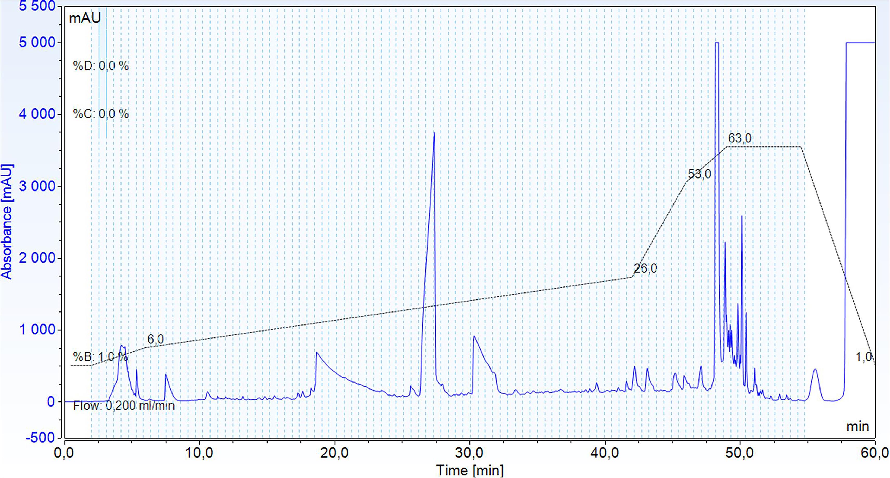
Figure 1. Example of a chromatogram showing the separation of TMT-labeled peptides during high pH reverse phase HPLC, monitored by absorbance at 214 nm (blue), and its gradient (black and dotted line). The light blue area depicts the sample collected in fractions, while the fractions are delimited by light blue and dotted lines.Collect 96 fractions of 100 μL in a ninety-six-well plate, starting at the minute 2.5 after injection.
Concatenate the ninety-six 100-μL fractions into 48 concatenated fractions by merging each fraction “n” with “n+48” (for example, 1 with 49, 2 with 50 … and 48 with 96).
Dry the final fractions using a speed-vacuum concentrator.
Inject the equivalent of 1 μg peptides of each fraction on a reversed-phase C18 nano-LC (nLC) column of a nano-LC–ESI–MS/MS instrument, with a C18 nano-trap column and the column for nLC separation at the temperature of 55 °C during peptide analysis.
Perform nLC separation using a binary solvent system, consisting of LC-MS buffer A and LC-MS buffer B, with a gradient of 4% to 26% B from 5 min to 91 min, 26% to 95% B in 9 min, and 5 min in 95% B, prior to equilibration in 4% A (Figure 2).
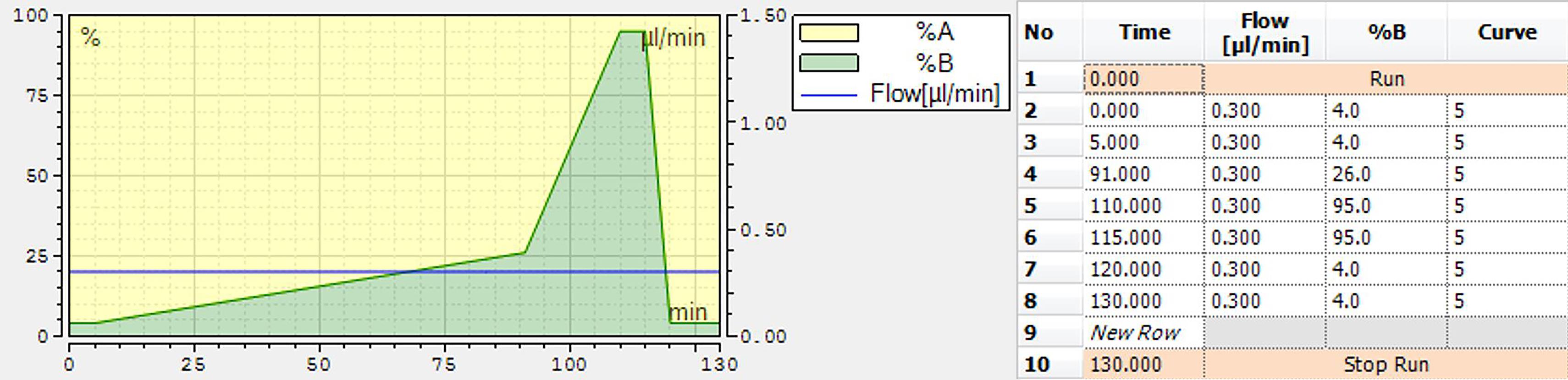
Figure 2. Gradient for nano-LC separation of TMT-labeled peptides before MS/MS analysisPerform quantitative bottom-up proteomics analysis for TMTpro-based MS/MS acquisition. Acquire mass spectra in a mass-to-charge (m/z) range of 375–1,500, with a resolution of 120 000 at m/z 200 for MS1. Set the AGC target to 3 × 10⁶, with a maximum injection time of 100 ms. Select the 17 most intense peptide peaks for peptide fragmentation via HCD, with the NCE value set at 33. The ion selection abundance threshold is set at 0.1% with charge exclusion of z = 1 ions. The MS/MS spectra are acquired at a resolution of 45 000, with an AGC target value of 2 × 10⁵ ions, or a maximum injection time of 120 ms. The fixed first m/z is 110, and the isolation window is 1.6 m/z. The instrument is operated in the positive ion mode for data-dependent acquisition of MS/MS spectra, with a dynamic exclusion time of previously selected precursor ions of 45 s.
Data analysis
Perform identification and quantification of peptides and proteins using MaxQuant or Proteome Discoverer (preferentially with the most recent versions of these software) as proteomic database search engine software. Search against the UniProt complete proteome database accordingly to the species of origin of the used cell culture (e.g., UP000005640 for human samples). When performing the database search for peptide and protein identification, use: cysteine carbamidomethylation as a fixed modification; TMT-related modifications; deamination on methionine oxidation, arginine, and asparagine as variable modifications; trypsin enzyme specificity with maximum of two missed cleavages. Use a 1% false discovery rate as a filter at both protein and peptide levels.
Remove all potential contaminants and reversed-hit peptides and include only proteins with at least two unique peptides in the quantitative analysis.
For analysis of the obtained protein data, eliminate the proteins with all missing values in all replicates in any treatment and normalize the quantified abundance of each protein in each sample (labeled with a different TMT) over the total intensity of all proteins for that sample.
For each protein in each replicate of D1–D5 ligands, divide the normalized protein abundance by the average abundance of this protein in the vehicle-treated replicates. Measure the average ratio across replicates of each D ligand/vehicle control and calculate the Log2 values of the obtained ratios.
Calculate the p-value for the assumption that the above ratio is non-zero using two-tailed Student’s t-test (with equal or unequal variance, depending on F test).
For each D ligand, visualize the results by a volcano plot containing the Log2 of the ratio as x-axis and -Log10 of the corresponding p-value as y-axis.
For each D ligand, the target candidates are found among the proteins with large absolute Log2 of the ratios and simultaneously large -Log10 of the p-values, also in comparison with what was obtained by the other D ligands, with potentially similar or different activities, induced phenotypes, or mechanisms.
Recipes
Cell lysis buffer
Reagent Final concentration Amount protease inhibitors (100×) 1× 150 μL PBS n/a 1,350 mL Total n/a 15 mL 20% NP40
Reagent Final concentration Amount NP40 (absolute) 20% 3 mL Milli-Q water n/a 12 mL Total n/a 15 mL 0.5 M DTT solution
Reagent Final concentration Amount DTT (absolute) 0.5 M 77 mg Milli-Q water n/a Add Milli-Q water to dissolve DTT until the volume is 1 mL Total n/a 1 mL 0.5 M IAA solution
Reagent Final concentration Amount IAA (absolute) 0.5 M 93 mg Milli-Q water n/a Add Milli-Q water to dissolve IAA until the volume is 1 mL Total n/a 1 mL 20 mM EPPS buffer (pH=8.2)
Reagent Final concentration Amount EPPS (absolute) 20 mM 250 mg Milli-Q water n/a Add 40 mL of Milli-Q water to dissolve EPPS 10 M NaOH solution n/a Adjust the pH until the final pH is 8.2 Milli-Q water n/a Add Milli-Q water until the volume is 50 mL Total n/a 50 mL 20 mM EPPS buffer (pH=8.2) including 8 M urea
Reagent Final concentration Amount Urea (absolute) 8 M 480 mg 20 mM EPPS buffer (pH=8.2) 20 mM Add Milli-Q water to dissolve urea until the volume is 1 mL Total n/a 1 mL 50% ACN solution
Reagent Final concentration Amount ACN (absolute) 50% (v/v) 25 mL Milli-Q water n/a 25 mL Total n/a 50 mL 0.1% TFA (v/v) solution
Reagent Final concentration Amount TFA (absolute) 0.1 % (v/v) 50 μL Milli-Q water n/a Add Milli-Q water until the volume is 50 mL Total n/a 50 mL 2% ACN (v/v) solution including 0.1% TFA
Reagent Final concentration Amount TFA (absolute) 0.1% (v/v) 50 μL ACN 2% (v/v) 1 mL Milli-Q water n/a Add Milli-Q water until the volume is 50 mL Total n/a 50 mL 2% ACN (v/v) solution including 0.1% FA (LC-MS buffer A)
Reagent Final concentration Amount Acetonitrile including 0.1% FA 2% 1 mL H2O including 0.1% FA n/a 49 mL Total n/a 50 mL 50% acetonitrile (v/v) solution including 0.1% FA
Reagent Final concentration Amount Acetonitrile including 0.1% FA 50 % 25 mL H2O including 0.1% FA n/a 25 mL Total n/a 50 mL 80% acetonitrile (v/v) solution including 0.1% FA
Reagent Final concentration Amount Acetonitrile including 0.1% FA 0.5 M 40 mL H2O including 0.1% FA n/a 10 mL Total n/a 50 mL 20 mM NH4OH in H2O (high pH Buffer A)
Reagent Final concentration Amount 28%–30% NH4OH water solution 20 mM 676 μL Milli-Q water n/a Add Milli-Q water until the volume is 500 mL Total n/a 500 mL 20 mM NH4OH in ACN (high pH Buffer B)
Reagent Final concentration Amount 28%–30% NH4OH water solution 20 mM 676 μL ACN n/a Add ACN to dissolve DTT to 500 mL Total n/a 500 mL 98% ACN in H2O including 0.1% FA (LC-MS buffer B)
Reagent Final concentration Amount Acetonitrile including 0.1% FA 98% 490 mL H2O including 0.1% FA n/a 10 mL Total n/a 500 mL
Acknowledgments
The PISA assay was invented, developed, and further optimized as method development of the Chemical Proteomics Core Facility of the Karolinska Institutet, Stockholm (https://ki.se/en/mbb/chemical-proteomics-core-facility), unique national unit of Chemical Proteomics at the Swedish infrastructures SciLifeLab (Science for Life Laboratrory, https://www.scilifelab.se/units/chemical-proteomics/), and BioMS (Swedish National Infrastructure for Biological Mass Spectrometry, https://bioms.se/technologies/chemical-proteomics/). The Chemical Proteomics Unit provides chemical proteomics support to research projects. SciLifeLab, BioMS, and Karolinska Insitutet supported this work.
This protocol was adapted from the original proof-of-principle article of the PISA method entitled “Proteome integral solubility alteration: a high-throughput proteomics assay for target deconvolution” (Gaetani et al., 2019).
Competing interests
The authors declare no competing interests.
Ethics
The protocol here described is generally applicable on any cell culture, commonly on commercial cell lines, and does not have any ethics requirement per se. It is to be noted that the protocol is also suitable to be applied to studies on primary cells extracted from human and/or animal tissues, and in such cases the use of cells derived from human or animal sources needs the approval by the ethics committee.
References
- Beusch, C. M., Sabatier, P. and Zubarev, R. A. (2022). Ion-Based Proteome-Integrated Solubility Alteration Assays for Systemwide Profiling of Protein–Molecule Interactions. Anal Chem 94(19): 7066-7074.
- Brenes, A., Hukelmann, J., Bensaddek, D. and Lamond, A. I. (2019). Multibatch TMT Reveals False Positives, Batch Effects and Missing Values*. Mol Cell Proteomics 18(10): 1967-1980.
- Chernobrovkin, A., Marin-Vicente, C., Visa, N. and Zubarev, R. A. (2015). Functional Identification of Target by Expression Proteomics (FITExP) reveals protein targets and highlights mechanisms of action of small molecule drugs. Sci Rep 5(1): 11176.
- Franken, H., Mathieson, T., Childs, D., Sweetman, G. M. A., Werner, T., Tögel, I., Doce, C., Gade, S., Bantscheff, M., Drewes, G., et al. (2015). Thermal proteome profiling for unbiased identification of direct and indirect drug targets using multiplexed quantitative mass spectrometry. Nat Protoc 10(10): 1567-1593.
- Gaetani, M., Sabatier, P., Saei, A. A., Beusch, C. M., Yang, Z., Lundström, S. L. and Zubarev, R. A. (2019). Proteome Integral Solubility Alteration: A High-Throughput Proteomics Assay for Target Deconvolution. J Proteome Res 18(11): 4027-4037.
- Gaetani, M. and Zubarev, R. A. (2019). Functional Identification of Target by Expression Proteomics (FITExP). Mass Spectrometry-Based Chemical Proteomics. 257-266.
- Heppler, L. N., Attarha, S., Persaud, R., Brown, J. I., Wang, P., Petrova, B., Tošić, I., Burton, F. B., Flamand, Y., Walker, S. R., et al. (2022). The antimicrobial drug pyrimethamine inhibits STAT3 transcriptional activity by targeting the enzyme dihydrofolate reductase. J Biol Chem 298(2): 101531.
- Kwon, H. J. and Karuso, P. (2018). Chemical proteomics, an integrated research engine for exploring drug-target-phenotype interactions. Proteome Science 16(1): 1.
- Lee, R. F. S., Chernobrovkin, A., Rutishauser, D., Allardyce, C. S., Hacker, D., Johnsson, K., Zubarev, R. A. and Dyson, P. J. (2017). Expression proteomics study to determine metallodrug targets and optimal drug combinations. Sci Rep 7(1): 1590.
- Li, J., Van Vranken, J. G., Paulo, J. A., Huttlin, E. L. and Gygi, S. P. (2020a). Selection of Heating Temperatures Improves the Sensitivity of the Proteome Integral Solubility Alteration Assay. J Proteome Res 19(5): 2159-2166.
- Li, J., Van Vranken, J. G., Pontano Vaites, L., Schweppe, D. K., Huttlin, E. L., Etienne, C., Nandhikonda, P., Viner, R., Robitaille, A. M., Thompson, A. H., et al. (2020b). TMTpro reagents: a set of isobaric labeling mass tags enables simultaneous proteome-wide measurements across 16 samples. Nat Methods 17(4): 399-404.
- Lin, A., Giuliano, C. J., Palladino, A., John, K. M., Abramowicz, C., Yuan, M. L., Sausville, E. L., Lukow, D. A., Liu, L., Chait, A. R., et al. (2019). Off-target toxicity is a common mechanism of action of cancer drugs undergoing clinical trials. 11(509): eaaw8412.
- Rix, U. and Superti-Furga, G. (2009). Target profiling of small molecules by chemical proteomics. Nat Chem Biol 5(9): 616-624.
- Sabatier, P., Beusch, C. M., Saei, A. A., Aoun, M., Moruzzi, N., Coelho, A., Leijten, N., Nordenskjöld, M., Micke, P., Maltseva, D., et al. (2021). An integrative proteomics method identifies a regulator of translation during stem cell maintenance and differentiation. Nature Communications 12(1): 6558.
- Saei, A. A., Beusch, C. M., Chernobrovkin, A., Sabatier, P., Zhang, B., Tokat, Ü. G., Stergiou, E., Gaetani, M., Végvári, Á. and Zubarev, R. A. (2019). ProTargetMiner as a proteome signature library of anticancer molecules for functional discovery. Nature Communications 10(1): 5715.
- Savitski, M. M., Reinhard, F. B. M., Franken, H., Werner, T., Savitski, M. F., Eberhard, D., Molina, D. M., Jafari, R., Dovega, R. B., Klaeger, S., et al. (2014). Tracking cancer drugs in living cells by thermal profiling of the proteome. 346(6205): 1255784.
- Swinney, D. C. and Anthony, J. (2011). How were new medicines discovered? Nature Reviews Drug Discovery 10(7): 507-519.
- Tarasova, N. K., Gallud, A., Ytterberg, A. J., Chernobrovkin, A., Aranzaes, J. R., Astruc, D., Antipov, A., Fedutik, Y., Fadeel, B. and Zubarev, R. A. (2017). Cytotoxic and Proinflammatory Effects of Metal-Based Nanoparticles on THP-1 Monocytes Characterized by Combined Proteomics Approaches. J Proteome Res 16(2): 689-697.
- Van Vranken, J. G., Li, J., Mitchell, D. C., Navarrete-Perea, J. and Gygi, S. P. (2021). Assessing target engagement using proteome-wide solvent shift assays. eLife 10: e70784.
- Wright, M. H. and Sieber, S. A. (2016). Chemical proteomics approaches for identifying the cellular targets of natural products. Nat Prod Rep 33(5): 681-708.
Article Information
Copyright
© 2022 The Authors; exclusive licensee Bio-protocol LLC.
How to cite
Readers should cite both the Bio-protocol article and the original research article where this protocol was used:
- Zhang, X., Lytovchenko, O., Lundström, S. L., Zubarev, R. A. and Gaetani, M. (2022). Proteome Integral Solubility Alteration (PISA) Assay in Mammalian Cells for Deep, High-Confidence, and High-Throughput Target Deconvolution. Bio-protocol 12(22): e4556. DOI: 10.21769/BioProtoc.4556.
- Heppler, L. N., Attarha, S., Persaud, R., Brown, J. I., Wang, P., Petrova, B., Tošić, I., Burton, F. B., Flamand, Y., Walker, S. R., et al. (2022). The antimicrobial drug pyrimethamine inhibits STAT3 transcriptional activity by targeting the enzyme dihydrofolate reductase. J Biol Chem 298(2): 101531.
Category
Systems Biology > Proteomics
Molecular Biology > Protein > Detection
Biochemistry > Protein > Quantification
Do you have any questions about this protocol?
Post your question to gather feedback from the community. We will also invite the authors of this article to respond.