Stimulus-induced Robust Narrow-band Gamma Oscillations in Human EEG Using Cartesian Gratings

Materials and Reagents

1. Setup for subjects’ seating area (Figure 1):

   1. Custom-designed chin rest (with mounted head rest).

   2. A table for stimulus presentation monitor (mentioned in the Equipment subsection) and chin rest.

   3. A stable chair for the subject to sit.

2. Inch tape (for measuring scalp diameter, as well as the distance between the monitor and the subject).

3. Personal items for cleaning the gel off scalp after the experiment, like tissue paper, towel, shampoo, etc.

   
   

   
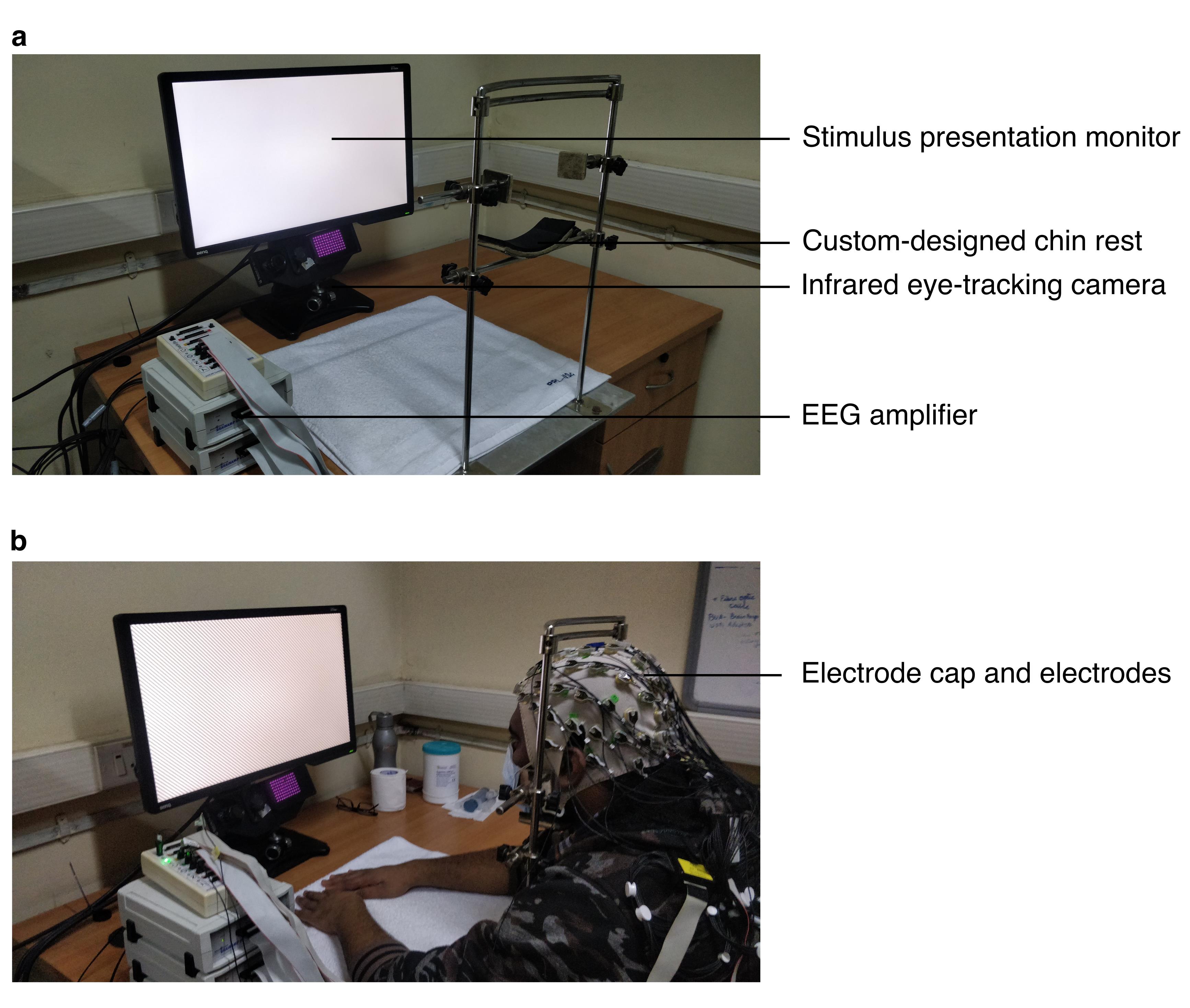
   Figure 1. Figure showing EEG setup in the subject area with and without the subject.

Equipment

1. EEG acquisition system

   1. Amplifier: BrainAmp DC (Brain Products GmbH, Germany)

   2. Electrodes: 64 active electrodes (Brain Products GmbH, Germany)

   3. Electrode cap: actiCAP (Easycap GmbH, Germany)

   4. Electrode gel: SuperVisc High Viscosity Electrolyte-Gel (Easycap GmbH, Germany)

   5. Recording computer: Windows PC with EEG recording software

2. Stimulus presentation monitor (in subject area): BenQ XL2411 (LCD, 1280×720 pixels, refresh rate: 100 Hz)

3. Monitor calibrating device (for gamma correction): i1Display Pro (X-Rite)

4. Eye-tracker: EyeLink 1000 (SR Research Ltd, Canada). This includes the infrared eye-tracking camera and the eye-data acquisition computer

5. Stimulus presentation computer: iMac (Mac OS X El Capitan)

Software

1. Stimulus presentation: custom library and app built in objective-c for Mac OS

2. EEG recording: Brain Vision Recorder (Version 1.20.0701)

3. Data analysis: MATLAB, with the following toolboxes/code:

   1. Chronux toolbox for signal processing

   2. Custom code (https://github.com/supratimray/TLSAEEGProjectPrograms) and EEGLAB for generating figures

Procedure

In the following sections, we describe in detail the procedure for EEG recording, artefact rejection, and data analysis used in Murty et al. (2020, 2021). These methods are built upon and have evolved from the methods that we used inMurty et al. (2018). For minor differences in these methods, we direct the readers to the original articles.

1. EEG room setup

   The experimenter’s rig comprised of a stimulus presentation computer, a recording computer, an analysis computer (optional), and an eye-data acquisition computer. The subject area was separated from the rig using thick curtains that also made sure that it was dark. Subjects sat on a stable chair and placed their chin on a chin rest. Their head was supported by cheek and head-rests mounted on the chin rest. We placed the gamma corrected monitor in front of and at the level of the chin rest, at a mean ± standard deviation (SD) distance of 58.1 ± 0.8 cm (range: 53.8–61.0 cm) from the subjects, according to their convenience. The monitor subtended a width of at least 52° and height of at least 30° of the visual field. The chin rest or its components never obstructed the monitor, and the entire monitor was always visible to the subjects. We calibrated the stimuli to the viewing distance for all subjects. We placed the eye-tracking camera below and at the center of the monitor. We instructed the subjects to wear spectacles, if prescribed.

2. EEG recording

   On the day of the experiment, we requested subjects to wash their hair with shampoo prior to coming for the recording session. We also briefed the subjects about the procedure and took their written consent before starting. Electrodes were placed on the scalp according to the international 10–10 system, using the electrode cap and gel as suggested by the manufacturer. We ensured that the gel under one electrode did not come in contact with the gel under another electrode. We also ensured that electrode impedances were less than 25 KΩ while applying gel, and rejected those electrodes that could not satisfy this criterion from analysis. After this process, we seated the subjects on the subject’s chair and calibrated the eye-tracker. We then presented a set of stimuli on the stimulus presentation monitor, while the subjects fixated on a small (0.1°) fixation point on the monitor. We acquired raw EEG signals by referencing all 64 electrodes to location ‘FCz’ on the scalp (see Figure 5). We filtered these signals online between 0.016 Hz (first-order filter) and 1000 Hz (fifth-order Butterworth filter), sampled at 2,500 Hz, and digitized at 16-bit resolution (0.1 μV/bit).

3. Stimuli

   Stimuli were static achromatic images whose luminosity varied sinusoidally across space, giving a sense of continuous, alternating black-and-white bars on the monitor. Such images are called gratings. These gratings are characterized by spatial frequency and orientation: spatial frequency is the frequency of the sinusoid (expressed as cycles per degree [cpd] of the visual field), and orientation is the direction perpendicular to the direction of the sinusoid (0° being vertical gratings). Gratings could further be varied in terms of their size (diameter) and contrast. We had observed that gratings with spatial frequency 1–4 cpd, having a diameter larger than 16° of visual field, and at 100% of contrast elicited robust slow and fast gamma oscillations in humans (Murty et al., 2018). Video 1 shows example full-screen stimuli (varied in spatial frequency and orientation) at 100% contrast.

   
   
   
   Video 1. Video showing example gratings and example trials.

   Each trial began with the appearance of a fixation point at the centre of the stimulus presentation screen. Within a trial, a series of gratings were presented (2 to 3 per trial) for 800 ms, with an interstimulus interval of 700 ms. Gratings were achromatic sinusoidal Cartesian gratings, whose spatial frequency was randomly chosen from 1, 2, and 4 cpd. The orientation of the gratings was randomly chosen from 0°, 45°, 90°, and 135°. The fixation point was presented on the screen throughout the trial, and disappeared at the end of the trial.

   
   

4. Stimulus presentation

   Details of stimulus presentation could be found in Murty et al. (2018, 2020, 2021). Example trials are shown in Video 1, and a video of a subject performing the task is shown in Video 2. Typically, the subjects fixated on the fixation point for 1,000 ms at the start of each trial. After this initial fixation period, we presented a series of gratings (2 to 3 per trial) for 800 ms, with an interstimulus interval of 700 ms. After the last stimulus of the trial was presented, the fixation point disappeared, and the subjects were allowed to rest their eyes by breaking fixation, while keeping their head stable. We performed each experiment in 1–2 blocks in a single session, according to the comfort of the subject. We gave breaks between blocks, during which the subjects could relax by removing their head off the chin rest. However, the distance of the chin rest from the monitor was kept constant between blocks. For a few subjects reported in Murty et al. (2018, 2020), we performed the experiments in two sessions according to the comfort of the subjects. For each session, we repeated the entire procedure of eye-tracker and stimulus calibration for monitor-to-chin rest distance.

   
   
   
   Video 2. Video of a subject performing the task.

   Subjects had to fixate on the fixation point throughout the trial. The trial was aborted if they broke fixation during the trial. After the trial ended or aborted, they were allowed to rest their eyes by breaking fixation, but keeping their head stable. Sounds were played through in-built speakers on iMac (the stimulus presentation computer) that alerted the subjects at the start of the trial, as well as when the trial ended, or when they broke fixation during the trial.

   
   

5. Data segmentation

   We first segmented EEG data between -1 to 2.2768 seconds around each stimulus onset time (total: 8192 points), and generated a N x 8192 data matrix for each electrode, where N is the number of stimulus repeats. Each segment is abbreviated as a “repeat”.

6. Artifact rejection

   We wanted to find a common set of bad repeats for all the electrodes, which would allow us to also do connectivity/causality analysis. In many cases, a small set of electrodes had a large number of bad repeats, so including those electrodes drastically reduced the total number of repeats for all electrodes. Therefore, we designed a fully automated artifact rejection pipeline to (i) find a set of bad electrodes, and (ii) a set of common bad repeats in the remaining good electrodes.

   As mentioned above, we rejected data offline from those electrodes whose impedance was more than 25 KΩ. We further rejected repeats with fixation breaks (defined as eye-blinks or shifts in eye-position outside a square window of width 5º, centered on the fixation spot) during 0.5s–0.75s of stimulus onset. We preprocessed the recorded data as follows (also described in Murty et al., 2020):

   1. For each unipolar electrode (Figure 2): We considered data for each electrode into smaller segments from -500 ms to 750 ms of stimulus onset. We then applied trial-wise thresholds in both time and frequency domain, as follows:

      1. For raw waveforms (time-domain): We first high-pass filtered the signal for each repeat at 1.6 Hz, to eliminate slow trends if any. We filtered the signal only for the purpose of artefact rejection, but not for final data analysis. Any stimulus repeat for which the filtered waveform deviated by six times the standard deviation (SD) from the mean at any time bin was considered as a bad repeat for that electrode.

      2. For Power Spectral Density (PSD; frequency-domain): We estimated multi-tapered PSDs from 0 to 200 Hz for each trial separately, with five tapers (time-bandwidth product or TW=3), using Chronux toolbox [(Mitra and Bokil, 2008), http://chronux.org/, RRID:SCR_005547]. Any stimulus repeat, for which the PSD deviated by 6 SD from the mean at any frequency point, was considered as a bad repeat for that electrode.

         
         

      
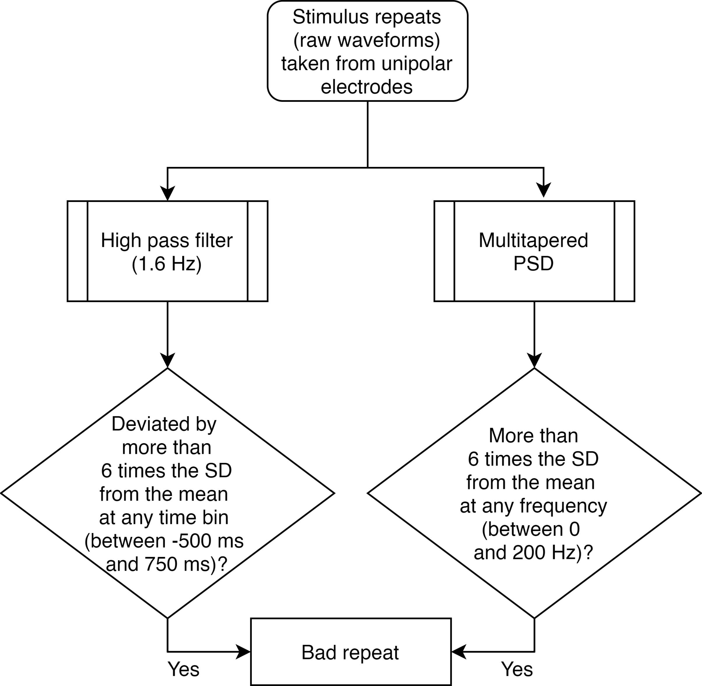
      Figure 2. Flowchart for separating bad repeats for each unipolar electrode.

      
      

   2. Common set of bad repeats (Figure 3): We next created a common set of bad repeats across all 64 unipolar electrodes, as follows:

      1. We first discarded those electrodes that had more than 30% of all repeats marked as bad (from step a).

      2. We then created a common set of bad repeats, by including in it any repeat (that was marked as bad in step a) in any of the ten unipolar electrodes used for analysis (P3, P1, P2, P4, PO3, POz, PO4, O1, Oz, and O2).

      3. Next, we included in this set any repeat (that was marked as bad in step a), if it occurred in more than 10% of the total number of remaining electrodes. This was the final set of bad repeats that we discarded, so the rest of the stimulus repeats were used for analysis.

         
         

      
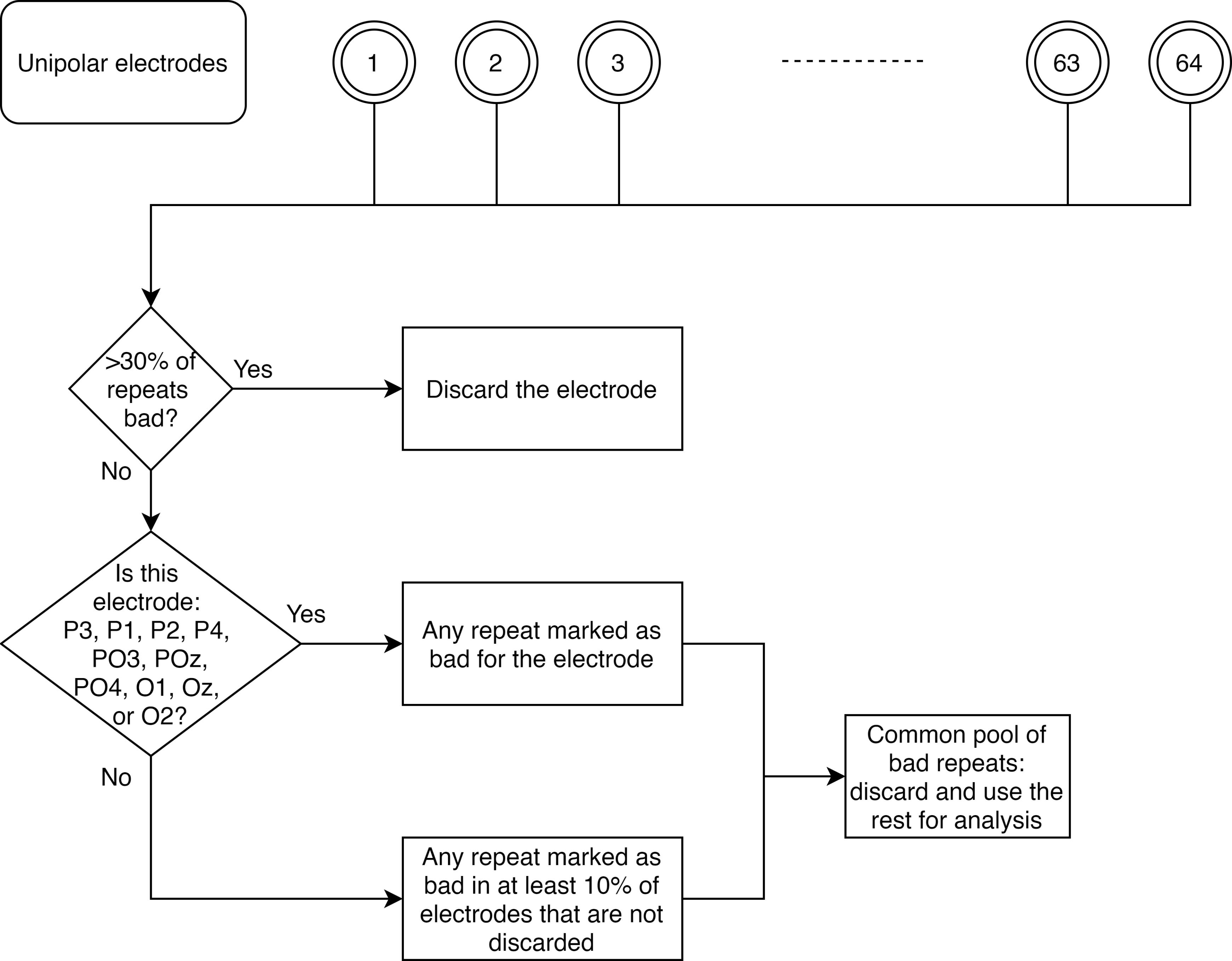
      Figure 3. Flowchart for creating a common set of bad repeats across all analyzable unipolar electrodes.

      
      

   3. Further rejection of electrodes (Figure 4): As mentioned above, we discarded those electrodes that had impedance more than 25 KΩ, or those that had more than 30% of all repeats marked as bad. Occasionally, we observed electrodes for which the PSD tended to flatten out (which could happen if it hit a noise floor, for example). We therefore added another pipeline to reject such electrodes. To this end, we calculated PSD slopes for each unipolar electrode, as follows:

      1. We estimated PSDs for each analyzable repeat using one taper (TW=1) and averaged the resulting PSDs.

      2. We fitted a power-law function, P(f)=A.f^-β to these trial-averaged PSDs, where A (scaling factor), and β (slope) are free parameters obtained using least square minimization (using the fminsearch function in MATLAB), and P is the PSD across frequencies f∈[56 84] Hz.

      We discarded those electrodes that had slopes less than 0. We did this separately for each block.

      
      

      
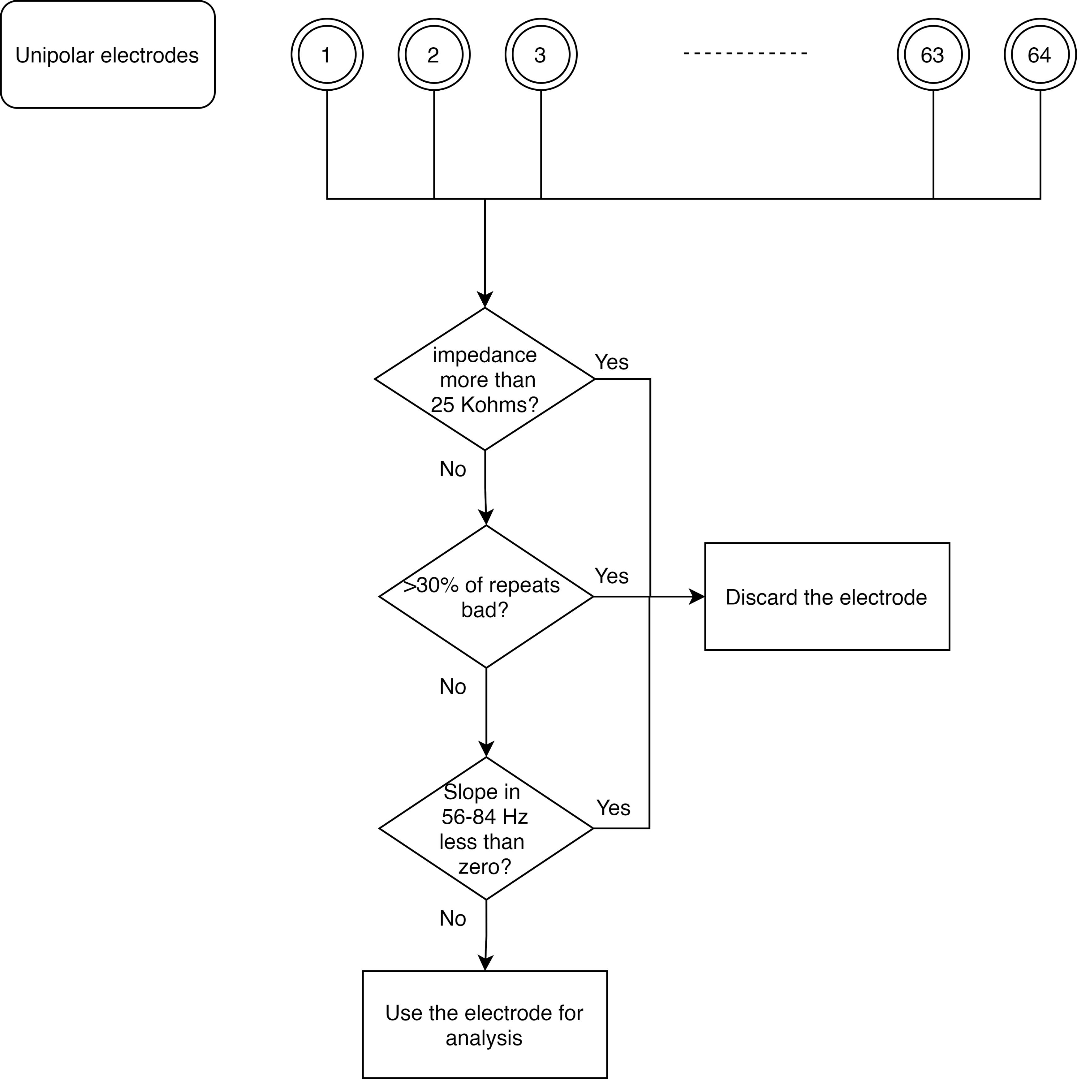
      Figure 4. Flowchart for discarding bad unipolar electrodes.

      
      

   For any block, if there were no analyzable bipolar electrodes (see Data Analysis subsection below), we discarded that block for that subject, and pooled the data across the rest of the blocks for data analysis. For minor differences in rejection of blocks for Murty et al. (2020, 2021), kindly refer to the respective articles.

   Data analysis

   1. Selection of electrodes

      We re-referenced data at each electrode offline to its neighboring electrodes (a reference scheme called bipolar reference), as shown in Figure 5 (Murty et al., 2020). This was done because we found that gamma oscillations were much more prominent in the bipolar referencing scheme (see Figure 1 of Murty et al., 2020). Specifically, we considered the following nine bipolar electrodes for analysis: PO3-P1, PO3-P3, POz-PO3, PO4-P2, PO4-P4, POz-PO4, Oz-POz, Oz-O1, and Oz-O2. We discarded a bipolar electrode if either of its constituting unipolar electrodes was marked bad during artifact rejection.

      
      

      
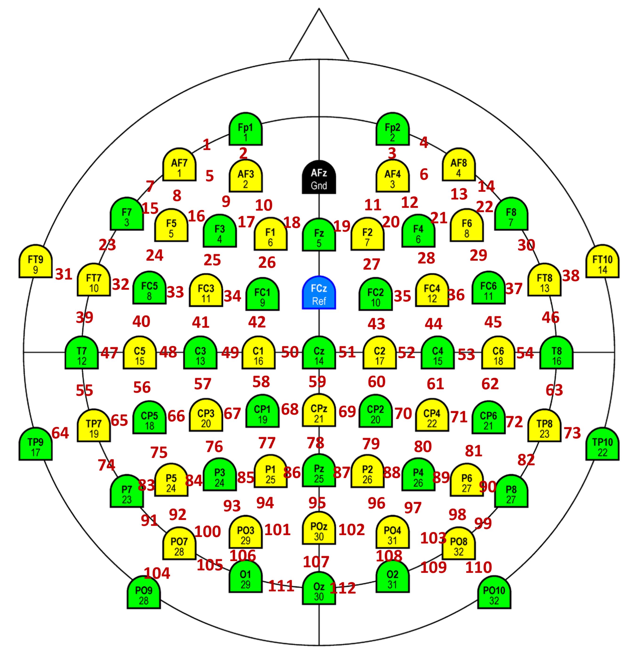
      Figure 5. Schematic showing bipolar montage. The colored electrodes are physical electrodes placed on the scalp, as per the International 10-10 System (Easycap GmbH, Germany). These electrodes are referenced online to FCz (unipolar reference scheme). Ground is at AFz. Data from adjacent physical electrodes are referenced offline with respect to each other (bipolar reference scheme). Bipolar electrodes are shown in red. Each bipolar electrode is virtually placed in between the two constituent unipolar electrodes. We analyzed 112 such electrodes in our studies.

      
      

   2. Analysis of EEG data

      We analyzed all data using custom codes written in MATLAB (The MathWorks, Inc., RRID:SCR_001622), as described inMurty et al. (2020). We computed PSD and the time-frequency power spectrograms using a multi-taper method with a single DPSS taper (TW=1), using the Chronux toolbox as described below. We averaged raw PSDs and raw spectrograms across all analyzable stimulus repeats for the final analysis. Further, we generated scalp maps using the topoplot.m function of EEGLAB toolbox (Delorme and Makeig, 2004, RRID:SCR_007292), modified to show each electrode as a colored disc.

      1. Computation of raw PSD and change in PSD: We calculated power at each frequency (at a resolution of 2 Hz) separately for the baseline period (−500 ms and 0 ms of stimulus onset), and stimulus period (250 ms and 750 ms, avoiding stimulus onset-related transients between 0 and 250 ms). For change in PSD from baseline to stimulus periods (expressed in dB), we used the following equation:

         
         

         

         
         

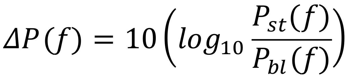
         where P(f) is the power at the frequency f. Figure 6a shows the raw PSD (black line) for stimulus (solid line), and baseline (dashed line) periods, as well as the change in PSD (blue solid line) for an example subject. Discernible gamma oscillations are observed as ‘bumps’ in 20-34 Hz (slow gamma), and 36-66 Hz (fast gamma) frequency ranges.

      2. Computation of raw and change in time-frequency power spectrograms: We estimated raw time-frequency power spectrograms during -500 ms and 1,200 ms of stimulus onset. We chose a moving window of 250 ms, and a step size of 25 ms, giving a frequency resolution of 4 Hz. For computation of change in the power spectrogram (expressed in dB), we subtracted the power averaged across the baseline period of the raw spectrogram from the entire raw spectrogram, for each frequency. In other words, we used the following formula:

         
         

         

         
         

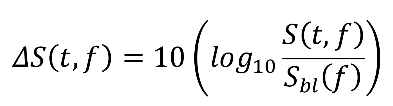
         where Sbl (f) is the baseline power at frequency (f) (averaged from -0.5 to 0 s). Figure 6b shows a raw spectrogram (top row) and a change in power spectrogram (bottom row), for the same example subject as in Figure 6a. Both slow and fast gamma oscillations are robustly observed in the change in power spectrogram.

      3. Computation of raw power in different frequency bands: To estimate raw power in frequency bands of interest (i.e., alpha, slow gamma and fast gamma) during baseline and stimulus periods, we summed the power at individual frequency bins in the respective frequency bands as estimated in the PSDs. In other words, we used the following equation:

         
         

         

         
         

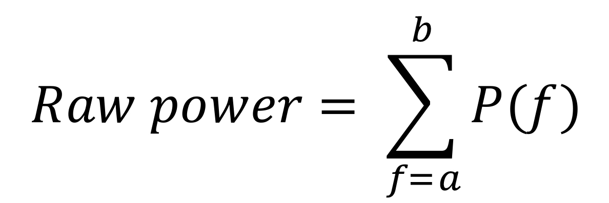
         where P(f) is the power at the frequency f, and a and b are the lower and upper limits of the frequency band of interest.

      4. Computation of stimulus-induced change in power in different frequency bands: To estimate the change in power during the stimulus period compared to the baseline period, we used the following equation for each frequency band:

         
         

         

         
         

      
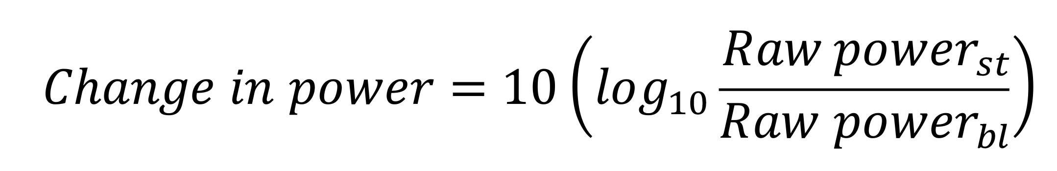
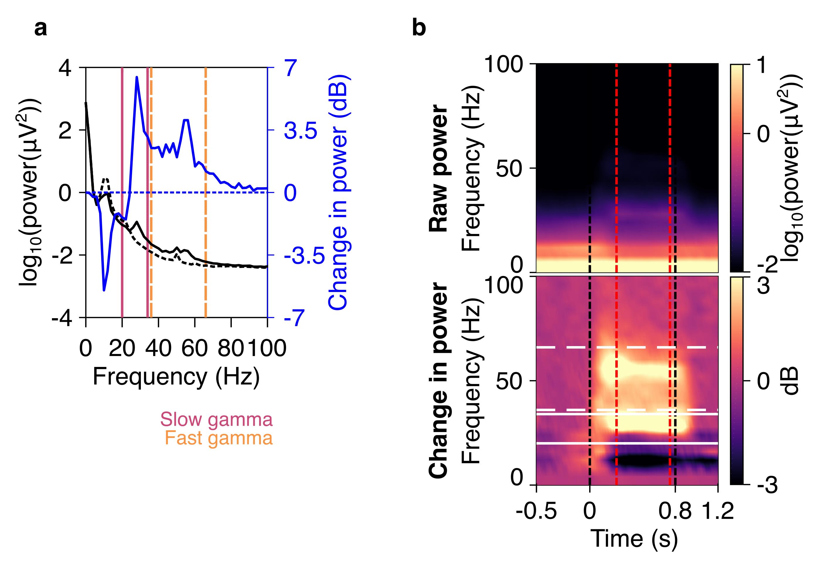
      Figure 6. Spectra and spectrograms in an example subject. a) Plot showing raw PSD (left axis) in the stimulus (black solid line) and baseline (black dashed line) periods, averaged across nine bipolar electrodes (PO3-P1, PO3-P3, POz-PO3, PO4-P2, PO4-P4, Poz-PO4, Oz-Poz, Oz-O1, and Oz-O2), and expressed on a log₁₀ scale. On the axis on the right side, the change in PSD (solid blue line) from stimulus to baseline periods is shown on a dB scale. Slow gamma (20–34 Hz) and fast gamma (36–66 Hz) bands are shown in vertical violet and orange lines respectively. b) A plot showing raw (top panel) and change in power time-frequency spectrograms (bottom panel), for the same data as in a. Gamma bands are shown in solid white (slow gamma), and dashed (fast gamma) lines. Vertical black dashed lines indicate the time when stimulus was presented to the subjects (0–0.8 s), whereas red vertical dashed lines indicate the stimulus period considered for spectral analysis (0.25–0.75 s).

      
      

   Codes for these analyses are available at: https://github.com/supratimray/TLSAEEGProjectPrograms.

   Codes for artifact rejection pipeline: https://github.com/supratimray/CommonPrograms under ReadData/findBadTrialsEEG.

   Acknowledgments

   This work was supported by Tata Trusts Grant, Wellcome Trust/DBT India Alliance (Intermediate fellowship 500145/Z/09/Z and Senior fellowship IA/S/18/2/504003 to SR), and DBT-IISc Partnership Programme (to SR). The original research article related to this protocol is as follows:

   Murty, D. V. P. S., Manikandan, K., Kumar, W. S., Ramesh, R. G., Purokayastha, S., Nagendra, B., Ml, A., Balakrishnan, A., Javali, M., Rao, N. P. and Ray, S. (2021). Stimulus-induced gamma rhythms are weaker in human elderly with mild cognitive impairment and Alzheimer's disease. Elife 10: e61666.

   Competing interests

   The authors declare no competing financial interests.

   Ethics

   All subjects participated in our studies voluntarily and were monetarily compensated for their time and effort. We obtained informed consent from all subjects before the experiment. The Institute Human Ethics Committees of Indian Institute of Science, NIMHANS, and M S Ramaiah Hospital, Bangalore approved all procedures.

   References

   1. Amir, A., Headley, D. B., Lee, S. C., Haufler, D. and Pare, D. (2018). Vigilance-Associated Gamma Oscillations Coordinate the Ensemble Activity of Basolateral Amygdala Neurons. Neuron 97(3): 656-669 e657.
   2. An, K. M., Ikeda, T., Yoshimura, Y., Hasegawa, C., Saito, D. N., Kumazaki, H., Hirosawa, T., Minabe, Y. and Kikuchi, M. (2018). Altered Gamma Oscillations during Motor Control in Children with Autism Spectrum Disorder. J Neurosci 38(36): 7878-7886.
   3. Buzsáki, G. and Wang, X. J. (2012). Mechanisms of gamma oscillations. Annu Rev Neurosci 35: 203-225.
   4. Chalk, M., Herrero, J. L., Gieselmann, M. A., Delicato, L. S., Gotthardt, S. and Thiele, A. (2010). Attention reduces stimulus-driven gamma frequency oscillations and spike field coherence in V1. Neuron 66(1): 114-125.
   5. Colgin, L. L., Denninger, T., Fyhn, M., Hafting, T., Bonnevie, T., Jensen, O., Moser, M. B. and Moser, E. I. (2009). Frequency of gamma oscillations routes flow of information in the hippocampus. Nature 462(7271): 353-357.
   6. Gieselmann, M. A. and Thiele, A. (2008). Comparison of spatial integration and surround suppression characteristics in spiking activity and the local field potential in macaque V1. Eur J Neurosci 28(3): 447-459.
   7. Gray, C. M., Konig, P., Engel, A. K. and Singer, W. (1989). Oscillatory responses in cat visual cortex exhibit inter-columnar synchronization which reflects global stimulus properties. Nature 338(6213): 334-337.
   8. Gregoriou, G. G., Gotts, S. J., Zhou, H. and Desimone, R. (2009). High-frequency, long-range coupling between prefrontal and visual cortex during attention. Science 324(5931): 1207-1210.
   9. Hirano, Y., Oribe, N., Kanba, S., Onitsuka, T., Nestor, P. G. and Spencer, K. M. (2015). Spontaneous Gamma Activity in Schizophrenia. JAMA Psychiatry 72(8): 813-821.
   10. Iaccarino, H. F., Singer, A. C., Martorell, A. J., Rudenko, A., Gao, F., Gillingham, T. Z., Mathys, H., Seo, J., Kritskiy, O., Abdurrob, F., et al. (2016). Gamma frequency entrainment attenuates amyloid load and modifies microglia. Nature 540(7632): 230-235.
   11. Juergens, E., Guettler, A. and Eckhorn, R. (1999). Visual stimulation elicits locked and induced gamma oscillations in monkey intracortical- and EEG-potentials, but not in human EEG. Exp Brain Res 129(2): 247-259.
   12. Kay, L. M. (2003). Two species of gamma oscillations in the olfactory bulb: dependence on behavioral state and synaptic interactions. J Integr Neurosci 2(1): 31-44.
   13. Koch, S. P., Werner, P., Steinbrink, J., Fries, P. and Obrig, H. (2009). Stimulus-induced and state-dependent sustained gamma activity is tightly coupled to the hemodynamic response in humans. J Neurosci 29(44): 13962-13970.
   14. Kumar, W. S., Manikandan, K., Murty, D. V. P. S., Ramesh, R. G., Purokayastha, S., Javali, M., Rao, N. P. and Ray, S. (2021). Stimulus-induced narrowband gamma oscillations are test-retest reliable in healthy elderly in human EEG. bioRxiv: 2021.2007.2006.451226.
   15. Mably, A. J. and Colgin, L. L. (2018). Gamma oscillations in cognitive disorders. Curr Opin Neurobiol 52: 182-187.
   16. Mitra, P. and Bokil, H. (2008). Observed brain dynamics. Oxford , New York: Oxford University Press.
   17. Murty, D. V. P. S., Manikandan, K., Kumar, W. S., Ramesh, R. G., Purokayastha, S., Nagendra, B., Ml, A., Balakrishnan, A., Javali, M., Rao, N. P. and Ray, S. (2021). Stimulus-induced gamma rhythms are weaker in human elderly with mild cognitive impairment and Alzheimer's disease. Elife 10: e61666.
   18. Murty, D. V. P. S., Manikandan, K., Kumar, W. S., Ramesh, R. G., Purokayastha, S., Javali, M., Rao, N. P. and Ray, S. (2020). Gamma oscillations weaken with age in healthy elderly in human EEG. Neuroimage 215: 116826.
   19. Murty, D. V. P. S., Shirhatti, V., Ravishankar, P. and Ray, S. (2018). Large Visual Stimuli Induce Two Distinct Gamma Oscillations in Primate Visual Cortex. J Neurosci 38(11): 2730-2744.
   20. Muthukumaraswamy, S. D. and Singh, K. D. (2013). Visual gamma oscillations: the effects of stimulus type, visual field coverage and stimulus motion on MEG and EEG recordings. Neuroimage 69: 223-230.
   21. Orekhova, E. V., Butorina, A. V., Sysoeva, O. V., Prokofyev, A. O., Nikolaeva, A. Y. and Stroganova, T. A. (2015). Frequency of gamma oscillations in humans is modulated by velocity of visual motion. Journal of Neurophysiology 114(1): 244-255.
   22. Palop, J. J. and Mucke, L. (2016). Network abnormalities and interneuron dysfunction in Alzheimer disease. Nat Rev Neurosci 17(12): 777-792.
   23. Pattisapu, S. and Ray, S. (2021). Stimulus-induced narrow-band gamma oscillations in humans can be recorded using open-hardware low-cost EEG amplifier. doi: https://doi.org/10.1101/2021.11.16.468841.
   24. Pesaran, B., Pezaris, J. S., Sahani, M., Mitra, P. P. and Andersen, R. A. (2002). Temporal structure in neuronal activity during working memory in macaque parietal cortex. Nat Neurosci 5(8): 805-811.
   25. Ray, S. and Maunsell, J. H. (2010). Differences in gamma frequencies across visual cortex restrict their possible use in computation. Neuron 67(5): 885-896.
   26. Ray, S. and Maunsell, J. H. (2011). Different origins of gamma rhythm and high-gamma activity in macaque visual cortex. PLoS Biol 9(4): e1000610.
   27. Shirhatti, V. and Ray, S. (2018). Long-wavelength (reddish) hues induce unusually large gamma oscillations in the primate primary visual cortex. Proc Natl Acad Sci U S A 115(17): 4489-4494.
   28. Siegel, M. and König, P. (2003). A functional gamma-band defined by stimulus-dependent synchronization in area 18 of awake behaving cats. J Neurosci 23(10): 4251-4260.
   29. Tada, M., Nagai, T., Kirihara, K., Koike, S., Suga, M., Araki, T., Kobayashi, T. and Kasai, K. (2016). Differential Alterations of Auditory Gamma Oscillatory Responses Between Pre-Onset High-Risk Individuals and First-Episode Schizophrenia. Cereb Cortex 26(3): 1027-1035.
   30. Uhlhaas, P. J. and Singer, W. (2007). What do disturbances in neural synchrony tell us about autism? Biol Psychiatry 62(3): 190-191.
   31. van Pelt, S. and Fries, P. (2013). Visual stimulus eccentricity affects human gamma peak frequency. Neuroimage 78: 439-447.
   32. Veit, J., Hakim, R., Jadi, M. P., Sejnowski, T. J. and Adesnik, H. (2017). Cortical gamma band synchronization through somatostatin interneurons. Nature Neuroscience 20(7): 951-959.
   33. Wilson, T. W., Rojas, D. C., Reite, M. L., Teale, P. D. and Rogers, S. J. (2007). Children and adolescents with autism exhibit reduced MEG steady-state gamma responses. Biol Psychiatry 62(3): 192-197.