Spatiotemporal Quantification of Cytosolic pH in Arabidopsis Pollen Tubes

Materials and Reagents

1. Safe-lock tubes, 1.5 ml (Eppendorf, catalog number: 0030120086)

2. Glass-bottom dishes (ThermoFisher Scientific, catalog number: 150680)

3. Glass microfiber filters (Sigma-Aldrich, catalog number: WHA1820047)

4. Potassium chloride (Sigma-Aldrich, catalog number: P9333)

5. Magnesium sulfate (Sigma-Aldrich, catalog number: 746452)

6. Boric acid (Sigma-Aldrich, catalog number: B6768)

7. Calcium chloride (Sigma-Aldrich, catalog number: C1016)

8. HEPES (Sigma-Aldrich, catalog number: H3375)

9. Sucrose (Sigma-Aldrich, catalog number: S7903)

10. Nigericin sodium salt (Tocris Bioscience, catalog number: 4312)

11. Sodium phosphate dibasic (Sigma-Aldrich, catalog number: S8282)

12. Sodium phosphate monobasic (Sigma-Aldrich, catalog number: S7907)

13. Agarose low gelling temperature (Sigma-Aldrich, catalog number: A9045)

14. Germination medium (see Recipe 1)

15. Stock solutions (see Recipe 2)

16. Sodium phosphate buffer (see Recipe 3)

17. Calibration solution (see Recipe 4)

Equipment

1. Hot plate

2. pH meter

3. Vortex

4. Fine needle-sharp tweezers (Sigma-Aldrich, catalog number: WHA1820047)

5. Benchtop microcentrifuge (Eppendorf, model: 5415D)

6. DeltaVision Imaging System (Applied Precision - GE, model: Elite)

   Note: Including an inverted microscope (Olympus, model: IX71), InsightSSI fluorescence illuminator, front-illuminated sCMOS camera (2560 × 2160, pixel size 6.45 μm), and 63 × 1.2 NA water immersion objective (Olympus, model: U-Plan S-Apo).

7. Filter sets, excitation 390/18 nm (DAPI) and 475/28 nm (FITC); emission, 435/48 nm (DAPI) and 523/36 nm (FITC)

8. Precise motorized X,Y stage

Software

1. ImageJ (Multiple Kymograph plugin), Fiji (https://imagej.net/Fiji/Downloads)

2. Statistical programming language R (R Core Team, 2020 – version 4.0.4 used here), RStudio recommended (RStudio Team, 2020 – version 1.4.1103 used here) and optionally, our custom-made analysis script CHUKNORRIS (Damineli et al., 2017)

3. Optional use of the custom R script ‘CalibrateFromKymographs.R’ supplied as Supplementary Material

Procedure

1. Pollen collection and sample preparation

   1. Prepare fresh liquid germination medium from stock solutions and adjust the pH to 7.5 (Recipe 1).

      Note: Store the stock solutions for the pollen germination medium at -20°C and prepare fresh germination medium on the day of the experiment.

   2. Grow Arabidopsis transgenic plants, expressing the ratiometric pHluorin under the LAT52 promoter (pLat52:pHluorin) (Hoffmann et al., 2020), in growth chambers under short-day photoperiod conditions (12 h light/12 h dark cycle) at 22°C with 70% humidity and a light intensity of ~100 μmol m^-2 s^−s to improve pollen integrity and density.

      Note: Growing Arabidopsis plants under short-day photoperiod conditions increases pollen quality and integrity, resulting in high germination rates (> 90%). Under these conditions, healthy plants take around 60 days to begin to flower. However, flowers grown under other photoperiod conditions can also be used.

   3. Collect flowers immediately after anthesis using thin tweezers and transfer to a 1.5-ml tube (no more than 100 flowers per tube – use 20-25 flowers per 10-mm dish).

      Notes:
      i) Start to collect flowers from the 10^th silique. The first siliques produced have reduced pollen density and the germination rate is reduced;

      ii) Collect flowers preferentially at 3-5 h of the light exposure cycle. After that, flowers start to close and pollen viability decreases;

      iii) Density is very important for Arabidopsis pollen germination. It is recommended that 20-25 flowers per 10-mm dish be collected. The parameter used here to standardize pollen density is the number of flowers; however, pollen density could vary according to growth chamber conditions. Of relevance, pollen grains should cover the glass-bottom dish, avoiding either sparse or overcrowded conditions.

   4. Add 1 ml germination liquid medium.

   5. Vortex at high speed (~2,500 rpm) for 30-40 s.

   6. Centrifuge at 1,600 × g for 3 min.

   7. Remove the flowers and supernatant.

   8. Resuspend gently the pollen precipitate in 100 μl liquid germination medium.

      Note: For pollen precipitate resuspension, cut off the first few millimeters of the 200-μl tip to enlarge the aperture and avoid pollen grain damage.

   9. Melt 0.01% low melting agarose in 1 ml germination medium in a safe-lock tube (1.5-ml) for 30 s in the microwave.

   10. Cool down the agarose enough to touch the tube with bare hands, without allowing it to jellify.

   11. Add 100 μl agarose solution to the pollen precipitate and mix gently.

   12. Add 50 μl solution (pollen grains in solution + jellified germination medium) to each glass-bottom dish (volume sufficient to prepare four experimental dishes).

   13. Place the glass-bottom dishes on a hot plate at 50°C for 1 min.

       Note: Pollen grains are sensitive to high temperatures and prolonged heat can kill them. Keep dishes under the heat for no longer than 2 min, just enough time to allow the pollen grains to sink to the glass bottom to facilitate imaging under the inverted microscope.

   14. Remove the dishes and allow the agarose solution to jellify.

       Note: The jellification of the germination medium containing pollen grains allows the pollen tubes to grow while enabling changes in the liquid solution on top. This step is fundamental for the calibration procedure.

   15. Add 100 μl liquid germination medium on top of the jellified agarose pad containing pollen grains.

   16. Incubate the dishes at 22°C, preferentially in the dark.

   17. After 2-3 h, growing pollen tubes with a length ≥ 200 μm can be assayed.

       Note: After 2-3 h of incubation, experimental dishes should be kept in an ice tray to slow pollen tube elongation from the beginning of image acquisition until the end of the procedure; otherwise, the tube will elongate continuously and after a few hours, the pollen tube length will be different from that acquired at the beginning of the procedure.

       
       Steps 1-17 are illustrated in Figure 1.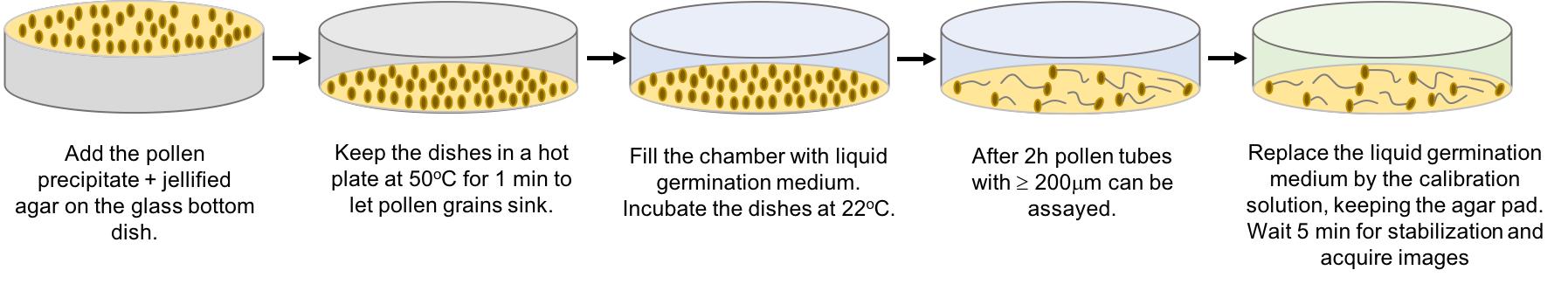

       
       

       
       Figure 1. Sample preparation procedure. Schematic illustration of the sequence steps for dish preparation and the pHluorin calibration procedure in Arabidopsis pollen tubes. The round drawing represents the 10-mm diameter well of the glass-bottom dish.

       
       

2. Calibration procedure and image acquisition

   1. Prepare 10 mM sodium phosphate buffer with molar ratios of mono- and dibasic forms appropriate for the following pHs: 5.8, 6.2, 6.6, 7.0, 7.4, 7.8, and 8.0; with 140 mM KCl and 30 µM nigericin (calibration solution – Recipes 3, 4 and Table 1).

      Note: Nigericin, a potassium ionophore that disrupts the membrane potential and intracellular H⁺ and K⁺ concentrations, is used to promote equilibrium between the pH in the cytosol and in the external solution.

   2. Remove the germination liquid medium from the dish with a pipette, retaining the agarose pad containing the growing pollen tubes.

   3. Add 100 μl of a given pH calibration solution.

   4. Wait 5 min for stabilization.

   5. Acquire time-lapse images of both channels (DAPI and FITC) every 4 s for 2 min for each growing pollen tube sampled at a given pH (Recipe 5).

      Notes:
      i) Apply the same acquisition protocol and microscope parameters to both experimental and calibration samples.

      ii) The Deltavision system was used to develop this protocol; however, the minimum imaging setup requirement to carry out the protocol would be any system capable of performing live-cell imaging with appropriate spatiotemporal resolution and timescales. Such a system should include an inverted microscope with a fluorescence source, a camera, and the appropriate emission/excitation filter set.

   6. Repeat steps 2-6 for all given pHs and replicates.

      Note: Acquire images of multiple tubes (10-20 replicates in individual tubes) at all pHs from at least two different dishes, but ideally three or more to avoid potential block effects.

      
      

      Table 1. Sodium phosphate buffer preparation from pH 5.8 to 8.0
      

      pH	Volume (ml) of 1 M Na2HPO4	Volume (ml) of 1 M NaH2PO4
      5.8	0.79	9.21
      6.2	1.78	8.22
      6.6	3.52	6.48
      7.0	5.77	4.23
      7.4	7.74	2.26
      7.8	8.96	1.04
      8.0	9.32	0.68

      
      

3. Kymograph extraction

   1. Generate kymographs from time-lapses.

      Watch a tutorial in Video 1.

      
      
      
      Video 1. Screen capture of the kymograph extraction procedure performed in ImageJ

      
      

   2. Open each file in ImageJ (Fiji recommended), splitting both DAPI and FITC channels.

   3. Trace a line along the midline of the pollen tube on the strongest channel using the 'segmented line' tool, starting from the shank and going to the tip. Make sure to extend the trace well beyond the pollen tube tip in order to sample enough background. It may be useful to start the trace at the last frame, for reference, and adjust the trace to make sure that it is roughly in the midline in every frame. Moreover, avoid the border of the shank with the observation window (Figure 2).

      
      

      
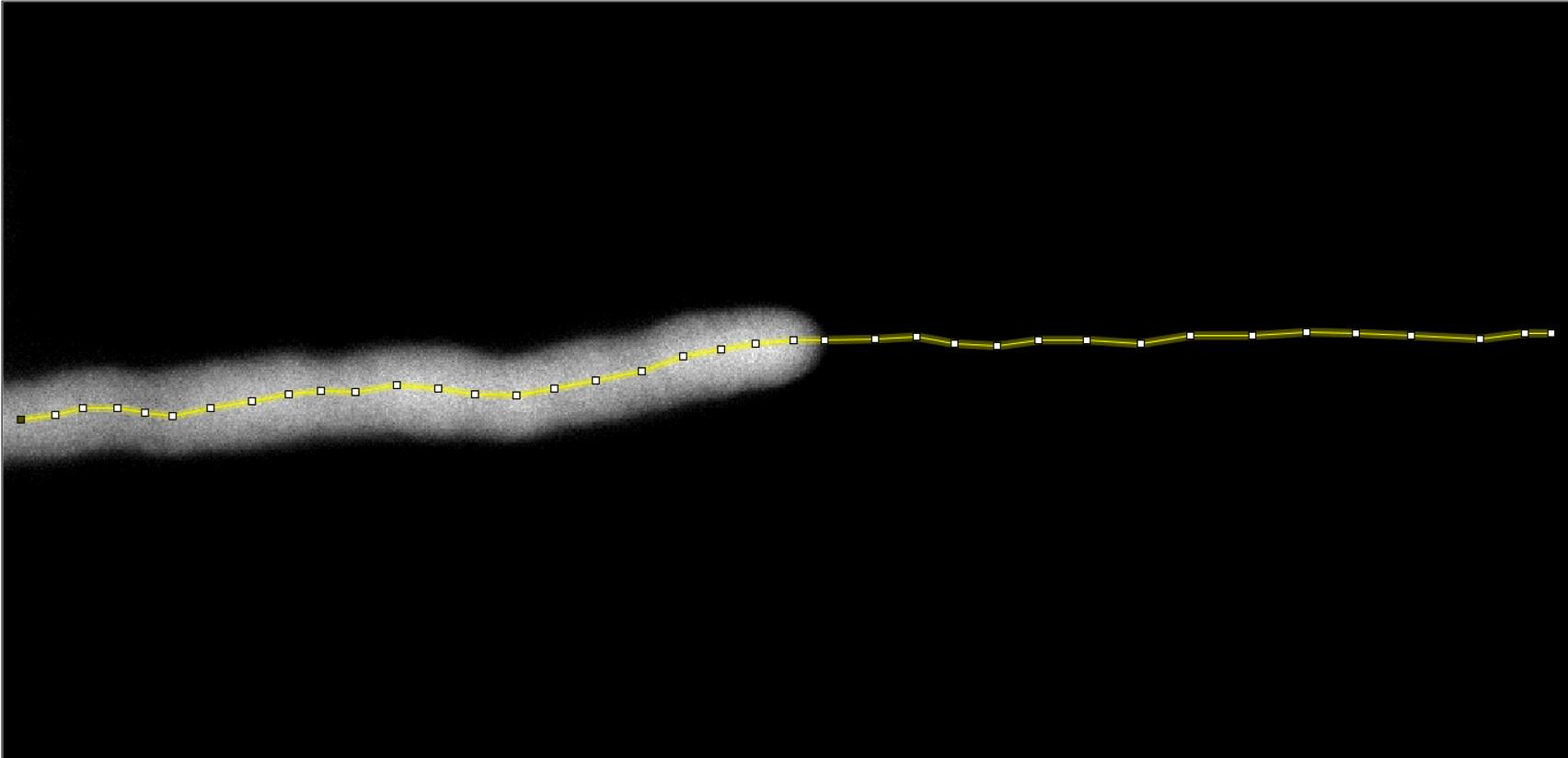
      Figure 2. Tracing for kymograph generation. Illustrative representation of the manual trace through the pollen tube midline drawn to generate the kymograph, using the Multiple kymograph plugin (ImageJ), averaging over a 7-pixel neighborhood along the trace for both pHluorin channels. Extending the trace out of the fluorescent image is fundamental to estimating the pixel intensity for background subtraction.

      
      

   4. Extract a kymograph along the midline, choosing a 7-pixel neighborhood using the 'Multiple Kymograph' plugin available under the Menu 'Analyze' in Fiji.

   5. Copy the line from one channel to the other using Command + Shift + E (on a Mac, replace ‘command’ with ‘control’ on Windows) and extract a kymograph as described in the previous step.

   6. Save each kymograph as text under 'File,' 'Save as,' 'Text Image.' To facilitate analysis, it is advisable to adopt a file-naming system; here, we recommend starting with the channel name and specifying the external pH and replicate number. Thus, each file acquired with the microscope will yield two kymographs named “FITC_5.8_1.txt” and “DAPI_ 5.8_1.txt,” in the case of the first replicate at pH 5.8. This file must have time as rows and space as columns, with the signal from the pollen tube on the left-hand side and the background on the right-hand side.

      
      

4. Data analysis

   1. Perform a linear regression of the ratio values as a function of external pH.
      Option 1: R script provided here that requires essentially no programming experience.

      Note: We exemplify the data analysis workflow using both data from Hoffmann et al. (2020) and surrogate data generated with the script “GenerateSurrogateData.R” provided as Supplementary Material. The surrogate data were generated to mimic kymographs used in the pH calibration, employing an asymptotic curve to represent the tip signal with added noise and actual pH values.

      
      

      Watch a tutorial in Video 2.

      
      Video 2. Screen capture of the calibration script performed in RStudio
      
      

      The supplementary R script “CalibrateFromKymographs.R” implements all the steps required to generate the calibration curve from the kymographs obtained at different external pHs, provided the file-naming system specified in Section C.6. is followed strictly. Any naming discrepancies will produce errors.

      1. Open RStudio and open the file ‘CalibrateFromKymographs.R’ through the menu “File” and “Open File…” The required parameters will be specified in the “User defined section” of the script.

      2. Specify where your files are located (‘fl.dir’) and where you want the output to be saved (‘out.dir’). Make sure the directory slash is in the correct orientation for your operating system: ‘/’ for MacOs and ‘\’ for Windows.

      3. Specify the name of the channel that is the denominator in calculating the ratio (‘top.ch’); here, it is ‘DAPI’ since we aim to calculate DAPI/FITC. This name must be exactly as in the prefix used to name the kymograph files, as explained in Section C.6. Any inconsistency will lead to errors.

      4. Choose the number of pixels to be used as a margin to calculate the background of each channel (‘mar’), counting from the tip location toward the right side of the matrix (see Figure 3A as a reference). This number cannot be larger than the distance from the furthest tip location to the end of the matrix; otherwise, it will cause an error.

      5. Choose the number of pixels to be used as a margin to define your region of interest behind the tip location and calculate the ratio signal (‘roi.mar’) counting from the tip location toward the left side of the matrix (see Figure 3A as a reference). This number cannot be larger than the shortest tip location plus the width defined in the next step.

      6. Define the width of your region of interest (‘roi.wdth’) in number of pixels, which will be placed behind the tip location estimate toward the left side of the matrix (see Figure 3A as a reference). This number cannot be larger than the shortest tip location plus the margin defined in the previous step.

      7. Watch the ‘KymoTimePoint’ plots (Figure 3A) in the output folder to see whether the tip location estimates seem adequate, that is, approximately locate the transition from signal to background. If not, one option is to set the fraction of the signal range used to automatically detect the tip (‘frac’) at a smaller value, if the location estimates are too far into the background region, or at a larger value, if the locations are found too far into the signal region.

      8. Make sure there is no significant trend in the median ratio signal over time (Figure 3B), which may suggest that the intracellular and extracellular concentrations did not equilibrate. See the ‘RatioInROI” plots in the output folder. If there is a consistent change over time, either discard the time points in the original file or discard the replicate.

      9. Click on “Source” on the top icons of the script and watch for errors, warnings, and messages on the ‘R Console.’

      10. Obtain the calibration curve in the output directory, which contains the estimated parameters, P-value, and R² in the legend (Figure 3C).

          
          

      
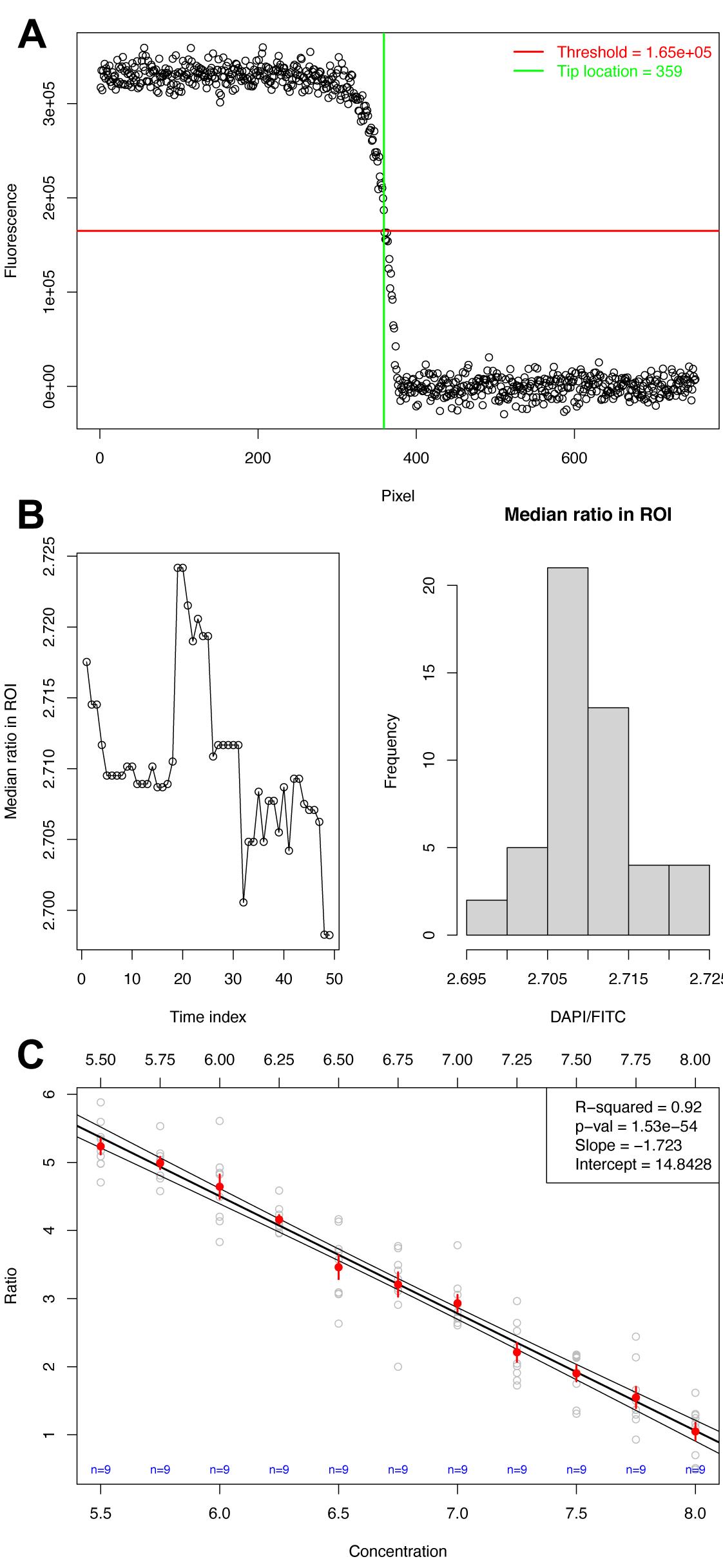
      Figure 3. Calibration of surrogate data mimicking pHluorin in Arabidopsis pollen tubes. A. Single timepoint where the tip location was estimated. B. Median ratio signal over time and overall distribution to verify whether there is a trend, plotted for each file in the output. C. Final calibration with coefficients and significance of the linear model.

      
      

   2. Linear regression Option 2: Custom R script that requires experience with programming. These are the steps implemented in Option 1 using the supplied script ‘CalibrateFromKymographs.R,’ but explained individually, allowing for greater flexibility in usage.

      1. Open the kymograph file in R (or Rstudio) using the function 'read.table.' This process will be described for a single file but can be easily automated.

      2. Estimate the boundary between the pollen tube tip and the background on the strongest channel either by using CHUKNORRIS (Damineli et al., 2017), the web app (https://feijolab.shinyapps.io/CHUK/), or simply with a threshold. The threshold value can be estimated visually by looking at which fluorescence value clearly separates signal from noise. Alternatively, one can attempt to automatically estimate the threshold, for example, as a fraction of the median signal range. To obtain the position (column) in the matrix 'm' at each time (row) where the pollen tube ends – for an arbitrary fluorescence threshold 'thrsh' – use 'apply(m, 1, function(v) max(which(v > thrsh))).'

      3. Estimate the median background value by subsetting the matrix 'm' after the position where the pollen tube ends on each row. This can be carried out in one command, for example, with 'median(unlist(lapply(pos, function(p) m[, (p+mar):dim(m)[2]]))),' where 'pos' is the vector of pollen tube tip positions obtained in the previous step, and 'mar' is an integer specifying the number of pixels to use as a margin (e.g., 5-25, depending on the number of pixels remaining to the right of each position).

      4. Estimate the signal value for that channel by averaging a region of a few pixels behind the pollen tube tip and subtracting the background.

      5. Open the file for the other channel and use the pollen tube tip position to estimate background (as in Section D.2.iii) and fluorescence signal (Section D.2.iv).

      6. Finally, calculate the ratio between the background-subtracted signal of each channel: pHluorin ratio = [(DAPI-DAPI_Background)/(FITC-FITC_Background)].

      7. Repeat D.2.i. - D.2.vi. for all other replicates and perform a linear model using 'lm,' where 'y' is the ratio values and 'x' is the extracellular pH (Figure 3C). Extract the coefficients for the slope and intercept and convert all ratio data into pH, provided that a satisfactory R² and p-value are attained. Typically, one expects a p-value well below 10^-2 and an R² above 0.5; although, one must check whether a linear fit looks like an appropriate description of the data. Alternatively, a sigmoidal fit may be more adequate, but that is outside the scope of this protocol.

   3. Use the linear model to estimate the real pH or concentration values.

      1. Now that a linear model has been fitted to the calibration data, one can estimate real values for the cytosolic concentration using an adapted equation for the line y=slope*x+intercept to yield pH:

         
         

         

         
         

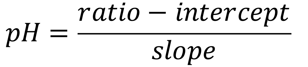
      2. Substitute the ratio values obtained from the desired experimental results in the equation above. If you extracted kymographs as in Section C.1. or as defined in Damineli et al. (2017) for your measurements of interest, this procedure allows a quantitative spatiotemporal estimate of pH (Figure 4) or other cytosolic concentrations.

      3. The intracellular gradient can be separately estimated as defined in Damineli et al. (2020).

         
         

      
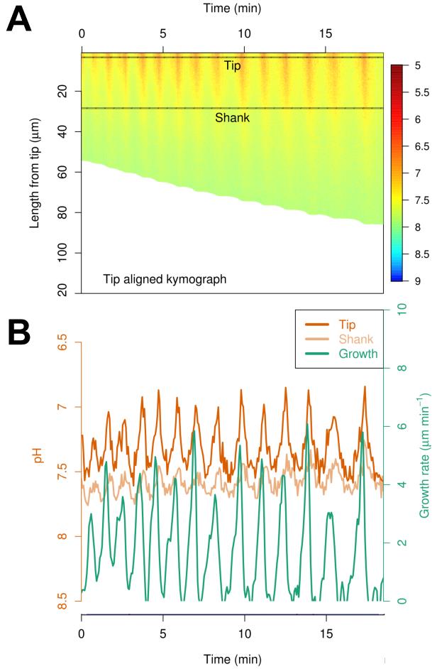
      Figure 4. Spatiotemporal quantification of cytosolic pH. A. Kymograph generated from ratiometric pHluorin calibration. B. Time series data from the aha6 aha8 mutant Arabidopsis pollen tubes presented in Hoffmann et al. (2020).

Recipes

1. Germination medium

   500 μM potassium chloride (KCl)

   500 μM calcium chloride (CaCl₂)

   125 μM magnesium sulfate (MgSO₄)

   0.005% (w/v) boric acid (H₃BO₃)

   125 μM 4-(2-hydroxyethyl)-1-piperazineethanesulfonic acid (HEPES)

   16% (w/v) sucrose

   Adjust pH to 7.5 with sodium hydroxide (NaOH)

2. Stock solutions

   Potassium chloride (KCl) 100 mM

   Calcium chloride (CaCl₂) 100 mM

   Magnesium sulphate (MgSO₄) 100 mM

   Boric acid (H₃BO₃) 1%

   4-(2-hydroxyethyl)-1-piperazineethanesulfonic acid (HEPES) 100 mM

3. Sodium phosphate buffer

   Prepare 1 M sodium phosphate dibasic (Na₂HPO₄)

   Prepare 1 M sodium phosphate monobasic (NaH₂PO₄)

4. Calibration solution

   10 mM sodium phosphate at the following pHs: 5.8, 6.2, 6.6, 7.0, 7.4, 7.8, 8.0

   140 mM KCl

   30 µM nigericin

5. Image acquisition protocol used in the Deltavision System

   Intensity: 10%

   Exposure time: 250 ms (for both channels)

   Channel 1: DAPI, FITC

   Channel 2: FITC, FITC

   Interval: 4 s

   Time-lapse: 16 points (64 s)

Acknowledgments

The J.F. lab was supported by National Science Foundation grants (MCB 1616437/2016 and 1930165/2019) and the University of Maryland. M.T.P. was funded by the grants 2019/26129-6 and 2021/05363-0 from the São Paulo Research Foundation (FAPESP). D.S.C.D. was funded by grants 19/23343-7 and 15/22308-2 from the São Paulo Research Foundation (FAPESP). We also acknowledge Majon et al. (2011) from where the protocol was adapted.

Competing interests

There are no conflicts of interest or competing interests.

References

1. Certal, A.C., Almeida, R.B., Carvalho, L.M., Wong, E., Moreno, N., Michard, E., Carneiro, J., Rodriguéz-Léon, J., Wu, H-M., Cheung, A.Y. and Feijó, J.A. (2008). Exclusion of a proton ATPase from the apical membrane is associated with cell polarity and tip growth in Nicotiana tabacum pollen tubes. Plant Cell 20: 614-634.
2. Choi, W-G., Toyota, M., Kim, S-H., Hilleary, R. and Gilroy, S. (2014). Salt stress-induced Ca²⁺ waves. Proc Natl Acad Sci U S A 111(17):6497-6502.
3. Damineli, D.S.C., Portes, M.T. and Feijó, J.A. (2017). Oscillatory signatures underlie growth regimes in Arabidopsis pollen tubes: computational methods to estimate tip location, periodicity, and synchronization in growing cells. J Exp Bot 68: 3267-3281.
4. Damineli, D. S. C., Portes, M. T. and Feijó, J. A. (2020). Analyzing intracellular gradients in pollen tubes. Methods Mol Biol 2160: 201-210.
5. Evans, M. J., Choi, W-G., Gilroy, S., Morris, R. J. (2016). A ROS-Assisted calcium wave dependent on the AtRBOHD NADPH oxidase and TPC1 cation channel propagates the systemic response to salt stress. Plant Physiol 171(3): 1771-1784.
6. Feijó, J. A. and Wudick, M. M. (2018). Calcium is life. J Exp Bot 69(17): 4147-4150.
7. Hilleary, R., Choi, W-G., Kim, S-H., Lim, S.D. and Gilroy, S. (2018). Sense and sensibility: the use of fluorescent protein-based genetically encoded biosensors in plants.Curr Opin Plant Biol 46: 32-38.
8. Hoffmann, R. D., Portes, M. T., Olsen, L. I., Damineli, D. S. C., Jesper, M. H., Pedersen, T., Lima, P. T. Campos, C., Feijó, J. A., Palmgren. M. (2020). Plasma membrane H⁺-ATPases sustain pollen tube growth and fertilization. Nat Comm 11: 2395.
9. Mahon, M. J. (2011). pHluorin2: an enhanced, ratiometric, pH-sensitive green florescent protein. Adv Biosci Biotechnol 2(3): 132-137.
10. Michard, E., Dias, P. and Feijó, J. A. (2008). Tobacco pollen tubes as cellular models for ion dynamics: improved spatial and temporal resolution of extracellular flux and free cytosolic concentration of calcium and protons using pHluorin and YC3.1 CaMeleon. Sex Plant Reprod 21: 169-181.
11. Miesenböck, G., De Angelis, D. A. and Rothman, J. E. (1998). Visualizing secretion and synaptic transmission with pH-sensitive green fluorescent proteins. Nature 394: 192–195.
12. Miyawaki, A., Llopis, J., Heim, R., McCaffery, J.M. and Adams, J. A., Ikura, M. and Tsien, R. Y. (1997). Fluorescent indicators for Ca²⁺ based on green fluorescent proteins and calmodulin. Nature 388: 882-887.
13. Monshausen, G. B., Messerli, M. A. and Gilroy, S. (2008). Imaging of the Yellow Cameleon 3.6 indicator reveals that elevations in cytosolic Ca²⁺ follow oscillating increases in growth in root hairs of Arabidopsis. Plant Physiol 147: 1690-1698.
14. Nagai, T., Yamada, S., Tominaga, T., Ichikawa, M. and Miyawaki, A. (2004). Expanded dynamic range of fluorescent indicators for Ca²⁺ by circularly permuted yellow fluorescent proteins. Proc Natl Acad Sci U S A 101: 10554-10559.
15. Ngo, Q.A., Vogler, H., Lituiev, D.S., Nestorova, A. and Grossniklaus, U. (2014). A calcium dialog mediated by the FERONIA signal transduction pathway controls plant sperm delivery. Dev Cell 29: 491-500.
16. Nguyen, C.T., Kurenda, A., Stolz, S., Chételat, A. and Farmer, E.E. (2018). Identification of cell populations necessary for leaf-to-leaf electrical signaling in a wounded plant. Proc Natl Acad Sci U S A 115(40): 10178-10183.
17. R Core Team. (2020). R: A language and environment for statistical computing. R Foundation for Statistical Computing, Vienna, Austria.
18. RStudio Team. (2020). RStudio: Integrated Development for R. RStudio, PBC, Boston, MA.
19. Toyota, M., Spencer, D., Sawai-Toyota, S., Jiaqi, W., Zhang, T., Koo, A. J., Howe, G. A. and Gilroy, S. (2018). Glutamate triggers long-distance, calcium-based plant defense signaling. Science 14: 1112-1115.
20. Walia, A., Waadt, R.and Jones, A.M. (2018). Genetically encoded biosensors in plants: pathways to discovery. Annu Rev Plant Biol 69(1): 497-524.