- Protocols

- Articles and Issues
- For Authors
- About
- Become a Reviewer

Detecting Differentially Methylated Promoters in Genes Related to Disease Phenotypes Using R
Published: Vol 11, Iss 11, Jun 5, 2021 DOI: 10.21769/BioProtoc.4033 Views: 4843
Reviewed by: Prashanth N SuravajhalaOctavio Morante-PalaciosErnesto Aparicio
Original research article
The authors used this protocol in:

Sep 2019
Advertisement


Protocol Collections
Comprehensive collections of detailed, peer-reviewed protocols focusing on specific topics


Abstract
DNA methylation in gene promoters plays a major role in gene expression regulation, and alterations in methylation patterns have been associated with several diseases. In this context, different software suites and statistical methods have been proposed to analyze differentially methylated positions and regions. Among them, the novel statistical method implemented in the mCSEA R package proposed a new framework to detect subtle, but consistent, methylation differences. Here, we provide an easy-to-use pipeline covering all the necessary steps to detect differentially methylated promoters with mCSEA from Illumina 450K and EPIC methylation BeadChips data. This protocol covers the download of data from public repositories, quality control, data filtering and normalization, estimation of cell type proportions, and statistical analysis. In addition, we show the procedure to compare disease vs. normal phenotypes, obtaining differentially methylated regions including promoters or CpG Islands. The entire protocol is based on R programming language, which can be used in any operating system and does not require advanced programming skills.
Keywords: MethylationBackground
DNA methylation plays an important role in many cellular processes and is currently being widely studied to gain a better understanding of human development and disease (Robertson, 2005). Most epigenome-wide association studies (EWAS) search for associations between DNA methylation and disease (Flanagan, 2015). For this aim, Illumina’s BeadChip arrays are widely used to measure DNA methylation in humans. Methylation in promoters is associated with gene expression repression (Boyes and Bird, 1992). The mechanisms of expression repression include impeding the binding of transcription factors and recruiting transcription repressors (Cedar and Bergman, 2012). Aberrant DNA methylation in these regions has been linked to several diseases, including cancer (Ehrlich and Lacey, 2013) and autoimmune disorders (Dozmorov et al., 2014). There are several R packages designed to detect differentially methylated regions that apply de novo and predefined strategies, as previously reviewed (Martorell-Marugán et al., 2019). Most of the predefined methods can be applied directly to detect differentially methylated promoters. On the contrary, de novo methods search for differentially methylated regions along the entire genome that should be annotated in order to detect which regions are located at promoters.
In this protocol, we present the complete data and statistical analysis pipeline to detect differentially methylated promoters in disease phenotypes from Illumina BeadChip data based on the mCSEA R package (Martorell-Marugán et al., 2019), which applies a predefined regions strategy. We used previously published data from patients with two rare neurodevelopmental diseases: Williams syndrome (WS) and 7q11.23 duplication syndrome (Dup7), as well as typically developing (TD) patients. Methylation in blood cells was measured in all the samples by the authors of the original study (Strong et al., 2015). This pipeline can be easily adapted to study other genomic regions such as gene body specific methylation patterns or CpG islands (CGIs). The complete code for this protocol is available as Supplemental_script file.
Equipment
Personal computer with Windows, MacOS, or Unix-based operating system
Software
R software environment 4.0.2. (https://www.r-project.org/)
RStudio integrated development environment 1.3.1056 (not required, but strongly recommended, https://rstudio.com/)
GEOquery R package 2.56.0 (Davis and Meltzer, 2007), https://www.bioconductor.org/packages/release/bioc/html/GEOquery.html
Minfi R package 1.34.0 (Aryee et al., 2014), https://www.bioconductor.org/packages/release/bioc/html/minfi.html
M3C R package 1.10.0 (John et al., 2020), https://www.bioconductor.org/packages/release/bioc/html/M3C.html
ggfortify R package 0.4.11 (Yuan et al., 2016), https://cran.r-project.org/web/packages/ggfortify/index.html
DMRcate R package 2.2.3 (Peters et al., 2015), https://www.bioconductor.org/packages/release/bioc/html/DMRcate.html
wateRmelon R package 1.32.0 (Pidsley et al., 2013), https://www.bioconductor.org/packages/release/bioc/html/wateRmelon.html
FlowSorted.Blood.450k R package 1.26.0, http://bioconductor.org/packages/release/data/experiment/html/FlowSorted.Blood.450k.html
mCSEA R package 1.8.0 (Martorell-Marugán et al., 2019), http://bioconductor.org/packages/release/bioc/html/mCSEA.html
Methylation data generated previously (Strong et al., 2015). GEO identifier: GSE66552 (https://www.ncbi.nlm.nih.gov/geo/query/acc.cgi?acc=GSE66552)
Procedure
Install the necessary R packages
The required packages to run this pipeline can be installed from CRAN and from Bioconductor repositories using the following commands in an R terminal:
install.packages("ggfortify")if (!requireNamespace("BiocManager", quietly = TRUE))
install.packages("BiocManager")
BiocManager::install(c("GEOquery", "minfi", "M3C", "DMRcate", "watermelon",
"FlowSorted.Blood.450k", "mCSEA"))
Download raw data
Figure 1 shows a diagram of the data analysis workflow. Illumina’s BeadChip arrays raw data are idat files containing the fluorescence intensities at each microarray spot. These idat files can be downloaded from the public Gene Expression Repository GEO (Edgar et al., 2002) using the GEOquery package (Davis and Meltzer, 2007). In this protocol, we are going to analyze data reported by Strong et al. (2015) that can be retrieved using the GEO identifier GSE66552. In an R session, execute the following code:
library(GEOquery)getGEOSuppFiles("GSE66552")
When the download finishes, there will be a folder in the current directory with the compressed data. Use this code to uncompress the data into the IDAT folder:
untar ("GSE66552/GSE66552_RAW.tar", exdir = "IDAT")Finally, save the metadata of the experiment into a variable called pheno:
GEOData <- getGEO("GSE66552")pheno <- pData(phenoData(GEOData[[1]]))
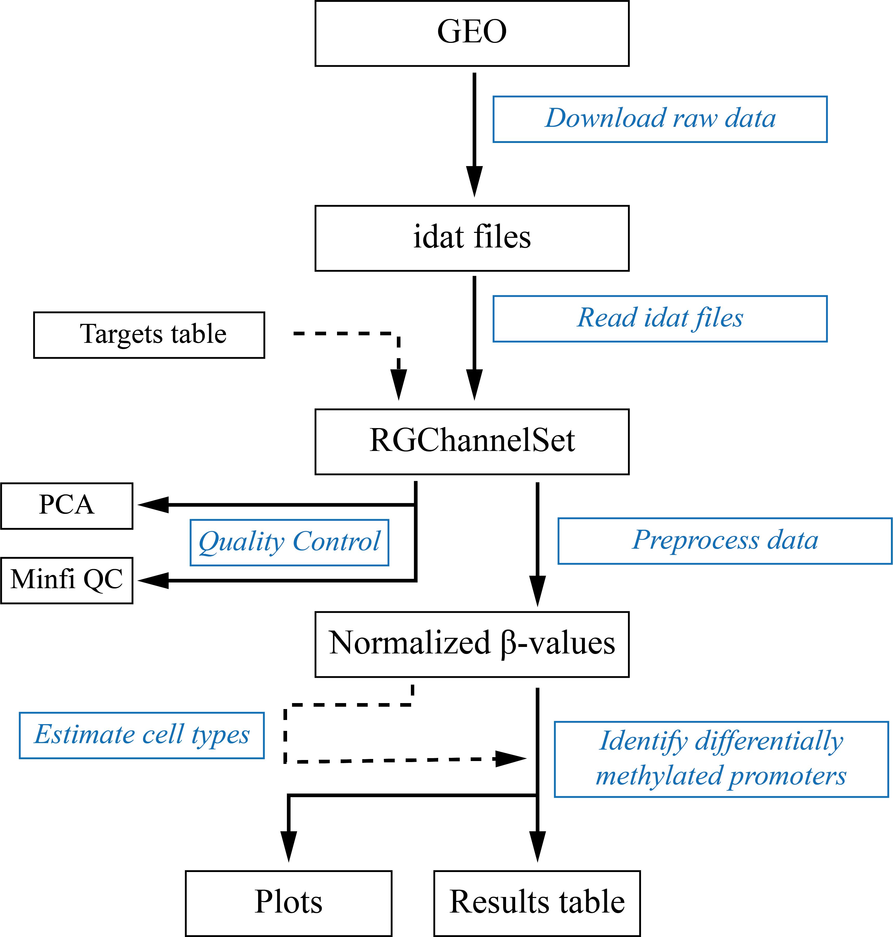
Figure 1. Data analysis workflow. Black boxes contain the inputs, outputs, and intermediate files. Blue boxes contain the steps described in this protocol.
Read idat files
Minfi package (Aryee et al., 2014) can be used to read the idat files and manipulate the methylation data. For this aim, a target dataframe should be created from the experiment metadata. Table 1 contains the first 5 rows of this dataset to show the structure that this object should have.
library(minfi)
basenames_split <- strsplit(pheno$supplementary_file, "suppl/")
basenames <- sapply(basenames_split, function(x) {return(x[2])})
targets <- data.frame("Sample_Name" = pheno$title, "Basename" = basenames)
Table 1. First 5 rows of the target dataframe
Sample_Name Basename TD control (Sample_1) GSM1624830_9376525009_R03C02_Grn.idat.gz TD control (Sample_2) GSM1624831_9376525033_R01C01_Grn.idat.gz WS (Sample_16) GSM1624832_8795207093_R01C01_Grn.idat.gz WS (Sample_17) GSM1624833_8795207093_R03C01_Grn.idat.gz WS (Sample_18) GSM1624834_8795207093_R04C01_Grn.idat.gz Read the data and store it in a RGChannelSet object that will be used for later analyses. RGChannelSet is the class used by minfi to store the raw methylation data. The sample names in this object may also be specified in this step.
rgchannelset <- read.metharray.exp(targets = targets, base = "IDAT")
sampleNames(rgchannelset) <- targets$Sample_Name
Perform quality control (QC)
To check that there are no technical problems affecting any samples, QC steps should be performed. Minfi package includes a function to explore the median intensities of unmethylated and methylated channels of each sample. Low intensities may indicate problems with a sample. Figure 2A shows the output plot of this QC. In this case, there are no samples failing this QC. If any sample fails this QC, it should be discarded from the analyses.
msetraw <- preprocessRaw(rgchannelset)
qc <- getQC(msetraw)
plotQC(qc)
Principal Components Analysis (PCA) is also a recommended QC step to detect potential outliers. To this end, M3C (John et al., 2020) and ggfortify (Yuan et al., 2016) R packages can be used. Figure 2B shows the PCA plot for our example. As can be observed, there are no outlier samples and the groups are partially separated. The observable mixing between groups may be due to covariates such as gender, age, or ancestry of the patients.
library(M3C)
library(ggfortify)
betas.raw <- getBeta(msetraw)
phenoPCA <- data.frame("Group" = pheno$`group:ch1`, stringsAsFactors = F)
pcaResult <- prcomp(t(na.omit(betas.raw)), scale. = TRUE)
autoplot(pcaResult, data = phenoPCA, colour = "Group")
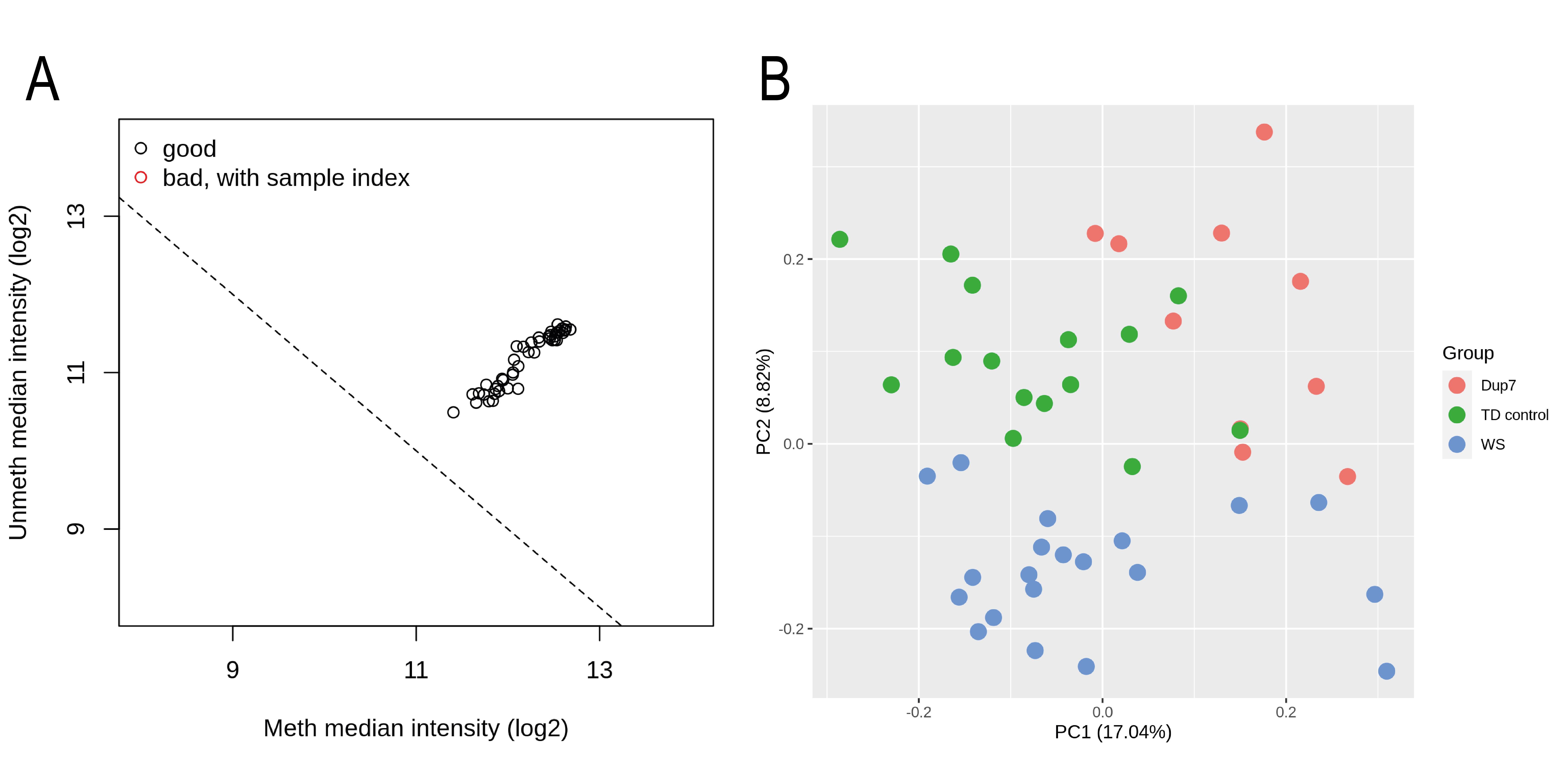
Figure 2. Quality control of methylation data. (A) Minfi QC with the median unmethylated and methylated signal intensities of each sample. (B) PCA plot representing the first two principal components. Samples are colored by experimental group.
Preprocess data
To correct for technical biases and improve the data quality, it is essential to filter some probes and apply normalization methods. Minfi preprocessNoob function applies Noob (normal-exponential out-of-band), a background correction with dye-bias normalization (Triche et al., 2013). The output of this normalization is a MethylSet object containing the methylated and unmethylated signals for each CpG probe. This object can be transformed to a RatioSet class where β-values are stored instead of signals. Finally, a GenomicRatioSet object containing the β-values mapped to the genome should be created. The GenomicRatioSet is the necessary class for further analyses.
mset <- preprocessNoob(rgchannelset)rset <- ratioConvert(mset)
grset <- mapToGenome(rset)
Subsequently, a detection P-value can be obtained for each probe and sample. This P-value is calculated by comparing the probe signal to the background signal measured using negative control probes. A detection P-value >0.01 indicates an untrustworthy signal. A filter step can be applied to remove those probes with a detection P-value >0.01 in a percentage of samples (in this case, at least 10% of samples).
detectionPvalues <- detectionP(rgchannelset)detectionPvalues <- detectionPvalues[rownames(grset),]
propGood <- apply(detectionPvalues, 1, function(x) {
length(x[which(x<0.01)])/ncol(detectionPvals)
})
grset <- grset[which(propGood >= 0.9),]
It is recommended to remove those probes that are located in sex chromosomes (only if both male and female samples are included) (Maksimovic et al., 2017), probes containing single nucleotide polymorphisms (SNPs) (Naeem et al., 2014), and cross-reactive probes (Chen et al., 2013). DMRCate package (Peters et al., 2015) contains the convenient function rmSNPandCH, which can be used to filter all these probes in one step:
library(DMRcate)beta.noob <- getBeta(grset)
beta.noob.filtered <- rmSNPandCH(beta.noob, rmXY = TRUE)
Finally, Beta-Mixture Quantile (BMIQ) normalization may be applied to mitigate the systematic differences between type I and type II probe designs present in 450K and EPIC arrays (Teschendorff et al., 2013). For this purpose, the wateRmelon package (Pidsley et al., 2013) may be used:
library(wateRmelon)annot <- getAnnotation(rgchannelset)
probeType <- as.data.frame(annot[rownames(beta.noob.filtered),c("Name","Type")])
probeType <- ifelse(probeType$Type %in% "I",1,2)
beta.normalized <- apply(beta.noob.filtered, 2, function(x) {
wateRmelon::BMIQ(x, design.v = probeType)$nbeta
})
Estimate cell type heterogeneity
One of the major sources of variability in blood methylation data is the different cell type proportions across samples (McGregor et al., 2016). In this context, reference data from the FlowSorted.Blood.450k package can be used to estimate these proportions in each sample. In the case of data generated with the EPIC platform, FlowSorted.Blood.EPIC package should be used instead.
library(FlowSorted.Blood.450k)
cellCounts <- estimateCellCounts(rgchannelset)
The cellCounts object is a matrix that can be merged with the experimental metadata to consider these estimations as covariates in further analyses:
pheno = merge(pheno, cellCounts, by.x = "title", by.y = "row.names")rownames(pheno) <- pheno$title
Identify differentially methylated promoters
One of the most common methylation analyses is to detect regions that show different methylation levels across phenotypes, known as Differentially Methylated Regions (DMRs). To this end, different statistical procedures have been developed, most of which are based on well-established methodologies such as linear models (Ritchie et al., 2015). In this protocol, we use the mCSEA package (Martorell-Marugán et al., 2019) to perform a DMRs analysis focusing on promoter regions. The first step is to rank CpG probes according to their differential methylation across conditions using linear models. In these models, available covariates (e.g., the estimated cell type proportions) can be included to adjust their possible effect on the data. Here, we are first analyzing the WS vs. TD control comparison:
library(mCSEA)
phenoComp <- pheno[,c("group:ch1","CD8T", "CD4T", "NK", "Bcell", "Mono", "Gran")]
rankedCpGs1 <- rankProbes(beta.normalized, phenoComp,
refGroup = "TD control", caseGroup = "WS",
covariates = c("CD8T", "CD4T", "NK", "Bcell", "Mono", "Gran"),
continuous = c("CD8T", "CD4T", "NK", "Bcell", "Mono", "Gran"))
The following step is used to calculate the differentially methylated promoters. The output object is a dataframe with gene symbols as row names, estimated P-values in the pval column, and P-values adjusted by the Benjamini-Hochberg method (Benjamini and Hochberg, 1995) in the padj column. In addition, given that the mCSEA algorithm is based on Gene Set Enrichment Analysis (GSEA) (Subramanian et al., 2005), the Enrichment Score (ES) is provided for each gene. The sign of this score indicates whether the promoter is hypermethylated (positive sign) or hypomethylated (negative sign) in the case group as compared with the controls. Finally, the Normalized ES (NES) and the amount of CpGs in each promoter are reported in the NES and size columns, respectively. Table 2 shows the first 20 rows of results_promoters1 object. In the case of EPIC data, the parameter platform = “EPIC” should be added to the mCSEATest function. Furthermore, the regionsTypes parameter can be modified to “genes” or “CGI” to analyze the gene bodies and CGIs, respectively.
set.seed(123)
results_mCSEA1 <- mCSEATest(rankedCpGs1, beta.normalized,
phenoComp, regionsTypes = "promoters")
results_promoters1 <- results_mCSEA1$promoters[order(results_mCSEA1$promoters$padj),
-c(3,7)]
Table 2. Top 20 differentially methylated promoters in WS vs. TD control comparison. Promoters are sorted by their adjusted P-value.
Gene P-value Adjusted P-value ES NES Size MYEOV2 1.00E-10 1.09E-07 -0.89 -3.18 26 KIAA1949 1.00E-10 1.09E-07 -0.65 -2.79 69 DDR1 1.02E-10 1.09E-07 -0.65 -2.69 56 FGF20 1.00E-10 1.09E-07 -0.97 -2.59 10 LOC650226 1.00E-10 1.09E-07 0.99 2.13 7 FLJ37307 1.00E-10 1.09E-07 0.99 2.14 7 HCN1 1.00E-10 1.09E-07 0.99 2.25 8 PRSS50 1.00E-10 1.09E-07 1.00 2.26 8 CRISP2 1.00E-10 1.09E-07 0.99 2.31 9 PRDM9 1.00E-10 1.09E-07 1.00 2.33 9 RBPJL 1.00E-10 1.09E-07 0.98 2.38 10 AURKC 1.00E-10 1.09E-07 0.95 2.39 11 PCDHB15 1.00E-10 1.09E-07 0.91 2.46 15 PLD6 1.00E-10 1.09E-07 0.99 2.63 14 HOXA4 1.00E-10 1.09E-07 0.87 2.67 24 DNAH6 1.25E-10 1.25E-07 0.94 2.43 12 ANKRD30B 3.07E-10 2.89E-07 0.91 2.43 14 HORMAD2 3.31E-10 2.94E-07 -0.92 -2.63 13 HOXB6 3.81E-10 3.21E-07 -0.76 -2.77 29 LYPD5 4.39E-10 3.52E-07 0.86 2.47 18 Perform the same analysis for Dup7 vs. TD control comparison:
rankedCpGs2 <- rankProbes(beta.normalized, phenoComp,refGroup = "TD control", caseGroup = "Dup7",
covariates = c("CD8T", "CD4T", "NK", "Bcell", "Mono", "Gran"),
continuous = c("CD8T", "CD4T", "NK", "Bcell", "Mono", "Gran"))
set.seed(123)
results_mCSEA2 <- mCSEATest(rankedCpGs2, beta.normalized,
phenoComp, regionsTypes = "promoters")
results_promoters2 <- results_mCSEA2$promoters[order(results_mCSEA2$promoters$padj),
-c(3,7)]
Furthermore, methylation values can be represented for any promoter in their genomic context. Figure 3A shows the result of this plot for the CRISP2 gene, whose promoter is hypermethylated in WS patients and hypomethylated in Dup7 patients. To construct these plots, use the mCSEAPlot function:
mCSEAPlot(results_mCSEA1, "promoters", "CRISP2", makePDF = F, leadingEdge = F)Finally, a GSEA plot can also be generated for each promoter. In this plot, all the analyzed CpGs are ordered by their differential methylation on the x axis, and vertical lines mark the CpGs belonging to the represented promoter. Figure 3B contains the CRISP2 GSEA plot, which can be generated with the mCSEAPlotGSEA function:
mCSEAPlotGSEA(rankedCpGs1, results_mCSEA1, "promoters", "CRISP2")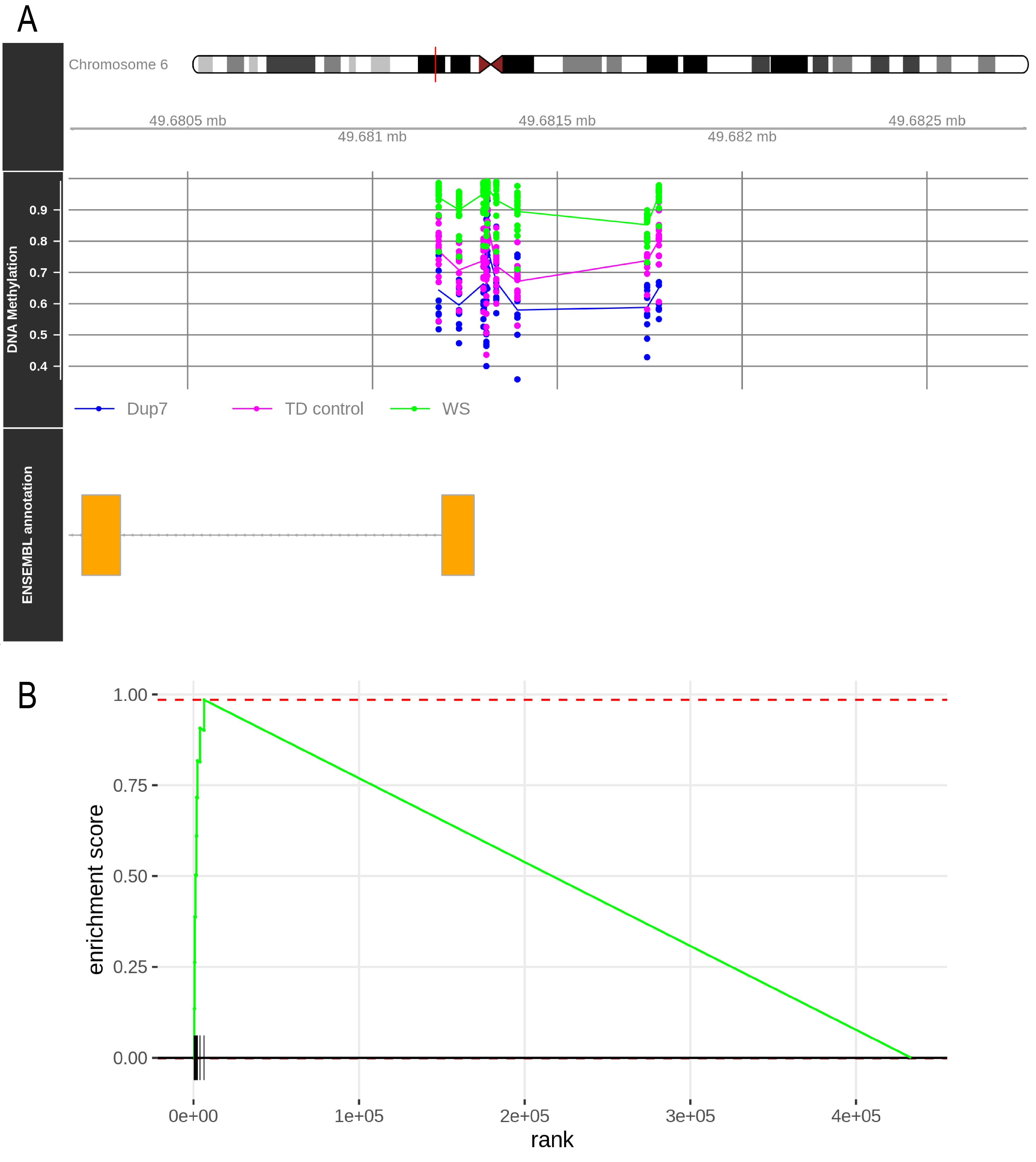
Figure 3. mCSEA plots for the CRISP2 gene. (A) Genomic context of the CRISP2 promoter. Points represent the β values for each CpG and sample. Lines show the mean methylation of each experimental group. (B) GSEA plot for the CRISP2 promoter in WS vs. TD control comparison. Vertical lines mark the location of CRISP2 promoter CpGs along the list of analyzed CpGs (horizontal black line).
Conclusions:
In this protocol, we show how to perform the whole analysis of Illumina BeadChip methylation data to identify differentially methylated promoters in disease samples using R packages. This protocol can be directly applied to any case-control study design. Furthermore, it can be easily adopted to study differential methylation in other regions such as gene bodies and CGIs. We are confident that this workflow will be useful for researchers studying methylation alterations associated with different disorders.
Acknowledgments
Jordi Martorell-Marugán is partially funded by Ministerio de Economía, Industria y Competitividad. This work was partially supported by FEDER/Junta de Andalucía-Consejería de Economía y Conocimiento (grant number: CV20-36723) and Consejería de Salud, Junta de Andalucía (Grant PI‐0173‐2017). We acknowledge the original research paper in which this protocol was derived (Martorell-Marugán et al., 2019).
Competing interests
The authors declare that they have no competing interests.
References
- Aryee, M.J., Jaffe, A.E., Corrada-Bravo, H., Ladd-Acosta, C., Feinberg, A.P., Hansen, K.D., and Irizarry, R.A. (2014). Minfi: a flexible and comprehensive Bioconductor package for the analysis of Infinium DNA methylation microarrays. Bioinformatics 30: 1363-1369.
- Benjamini, Y., and Hochberg, Y. (1995). Controlling the false discovery rate: A practical and powerful approach to multiple testing. J R Stat Soc 57: 289-300.
- Boyes, J., and Bird, A. (1992). Repression of genes by DNA methylation depends on CpG density and promoter strength: evidence for involvement of a methyl-CpG binding protein. EMBO J 11(1): 327-333.
- Cedar, H., and Bergman, Y. (2012). Programming of DNA Methylation Patterns. Annu Rev Biochem 81: 97-117.
- Chen, Y., Lemire, M., Choufani, S., Butcher, D.T., Grafodatskaya, D., Zanke, B.W., Gallinger, S., Hudson, T.J., and Weksberg, R. (2013). Discovery of cross-reactive probes and polymorphic CpGs in the Illumina Infinium HumanMethylation450 microarray. Epigenetics 8: 203-209.
- Davis, S., and Meltzer, P.S. (2007). GEOquery: a bridge between the Gene Expression Omnibus (GEO) and BioConductor. Bioinformatics 23: 1846-1847.
- Dozmorov, M.G., Wren, J.D., and Alarcón-Riquelme, M.E. (2014). Epigenomic elements enriched in the promoters of autoimmunity susceptibility genes. Epigenetics 9: 276-285.
- Edgar, R., Domrachev, M., and Lash, A.E. (2002). Gene Expression Omnibus: NCBI gene expression and hybridization array data repository. Nucleic Acids Res 30: 207-210.
- Ehrlich, M., and Lacey, M. (2013). DNA Hypomethylation and Hemimethylation in Cancer. Adv Exp Med Biol 754:31-56.
- Flanagan, J.M. (2015). Epigenome-wide association studies (EWAS): past, present, and future. Methods Mol Biol Clifton NJ 1238: 51-63.
- John, C.R., Watson, D., Russ, D., Goldmann, K., Ehrenstein, M., Pitzalis, C., Lewis, M., and Barnes, M. (2020). M3C: Monte Carlo reference-based consensus clustering. Sci Rep 10: 1816.
- Maksimovic, J., Phipson, B., and Oshlack, A. (2016). A cross-package Bioconductor workflow for analysing methylation array data. F1000Res 5: 1281.
- Martorell-Marugán, J., González-Rumayor, V., and Carmona-Sáez, P. (2019). mCSEA: detecting subtle differentially methylated regions. Bioinforma Oxf Engl 35: 3257-3262.
- McGregor, K., Bernatsky, S., Colmegna, I., Hudson, M., Pastinen, T., Labbe, A., and Greenwood, C.M.T. (2016). An evaluation of methods correcting for cell-type heterogeneity in DNA methylation studies. Genome Biol 17: 84.
- Naeem, H., Wong, N.C., Chatterton, Z., Hong, M.K.H., Pedersen, J.S., Corcoran, N.M., Hovens, C.M., and Macintyre, G. (2014). Reducing the risk of false discovery enabling identification of biologically significant genome-wide methylation status using the HumanMethylation450 array. BMC Genomics 15: 51.
- Peters, T.J., Buckley, M.J., Statham, A.L., Pidsley, R., Samaras, K., V Lord, R., Clark, S.J., and Molloy, P.L. (2015). De novo identification of differentially methylated regions in the human genome. Epigenetics Chromatin 8: 6.
- Pidsley, R., Y Wong, C.C., Volta, M., Lunnon, K., Mill, J., and Schalkwyk, L.C. (2013). A data-driven approach to preprocessing Illumina 450K methylation array data. BMC Genomics 14: 293.
- Ritchie, M.E., Phipson, B., Wu, D., Hu, Y., Law, C.W., Shi, W., and Smyth, G.K. (2015). limma powers differential expression analyses for RNA-sequencing and microarray studies.Nucleic Acids Res 43: e47-e47.
- Robertson, K.D. (2005). DNA methylation and human disease. Nat Rev Genet 6: 597-610.
- Strong, E., Butcher, D.T., Singhania, R., Mervis, C.B., Morris, C.A., De Carvalho, D., Weksberg, R., and Osborne, L.R. (2015). Symmetrical Dose-Dependent DNA-Methylation Profiles in Children with Deletion or Duplication of 7q11.23. Am J Hum Genet 97: 216-227.
- Subramanian, A., Tamayo, P., Mootha, V.K., Mukherjee, S., Ebert, B.L., Gillette, M.A., Paulovich, A., Pomeroy, S.L., Golub, T.R., Lander, E.S., et al. (2005). Gene set enrichment analysis: A knowledge-based approach for interpreting genome-wide expression profiles. Proc Natl Acad Sci 102: 15545-15550.
- Teh, A.L., Pan, H., Lin, X., Lim, Y.I., Patro, C.P.K., Cheong, C.Y., Gong, M., MacIsaac, J.L., Kwoh, C.-K., Meaney, M.J., et al. (2016). Comparison of Methyl-capture Sequencing vs. Infinium 450K methylation array for methylome analysis in clinical samples. Epigenetics 11: 36-48.
- Teschendorff, A.E., Marabita, F., Lechner, M., Bartlett, T., Tegner, J., Gomez-Cabrero, D., and Beck, S. (2013). A beta-mixture quantile normalization method for correcting probe design bias in Illumina Infinium 450 k DNA methylation data. Bioinforma Oxf Engl 29: 189-196.
- Triche, T.J., Weisenberger, D.J., Van Den Berg, D., Laird, P.W., and Siegmund, K.D. (2013). Low-level processing of Illumina Infinium DNA Methylation BeadArrays. Nucleic Acids Res 41: e90-e90.
- Yuan, T., Horikoshi, M., and Li, W. (2016). ggfortify: Unified Interface to Visualize Statistical Results of Popular R Packages. R J 8: 474-485.
Article Information
Copyright
© 2021 The Authors; exclusive licensee Bio-protocol LLC.
How to cite
Martorell-Marugán, J. and Carmona-Sáez, P. (2021). Detecting Differentially Methylated Promoters in Genes Related to Disease Phenotypes Using R. Bio-protocol 11(11): e4033. DOI: 10.21769/BioProtoc.4033.
Category
Systems Biology > Epigenomics > DNA methylation
Systems Biology > Genomics
Do you have any questions about this protocol?
Post your question to gather feedback from the community. We will also invite the authors of this article to respond.