- Protocols

- Articles and Issues
- For Authors
- About
- Become a Reviewer

sc3D: A Comprehensive Tool for 3D Spatial Transcriptomic Analysis
Published: Vol 16, Iss 4, Feb 20, 2026 DOI: 10.21769/BioProtoc.5607 Views: 688
Reviewed by: Navnita DuttaAnonymous reviewer(s)
Original research article
The authors used this protocol in:

Jul 2023
Advertisement


Protocol Collections
Comprehensive collections of detailed, peer-reviewed protocols focusing on specific topics


Abstract
Serial spatial omics technologies capture genome-wide gene expression patterns in thin tissue sections but lose spatial continuity along the third dimension. Reconstructing these two-dimensional measurements into coherent three-dimensional volumes is necessary to relate molecular domains, gradients, and tissue architecture within whole organs or embryos. sc3D is an open-source Python framework that registers consecutive spatial transcriptomic sections, interpolates bead coordinates in three dimensions, and stores the result in an AnnData object compatible with Scanpy. The workflow performs slice alignment, 3D reconstruction, optional downsampling, and interactive visualization in a napari-sc3D-viewer, enabling virtual in situ hybridization and spatial differential gene expression analysis. We tested sc3D on Slide-seq and Stereo-seq datasets, including E8.5 and E16.5 mouse embryos, recovering continuous tissue morphologies, cardiac anatomical markers, and the expected anterior–posterior gradients of Hox gene expression. These results show that sc3D allows reproducible reconstruction and analysis of volumetric spatial omics data across different samples and experimental platforms.
Key features
• 3D reconstruction: sc3D aligns serial Slide-seq arrays and interpolates between sections to generate volumetric transcriptomic datasets preserving tissue geometries.
• Portable data formats: Outputs a .h5ad object storing coordinates, expression, and metadata, readable in Python or napari-sc3D-viewer.
• Integrated visualization: The napari plugin enables interactive 3D exploration, virtual in situ hybridization, and gene expression profiling along developmental axes.
• Spatial differential expression: Built-in functions detect regionally enriched genes and export quantitative 3D heatmaps and ranked tables.
Keywords: sc3DGraphical overview
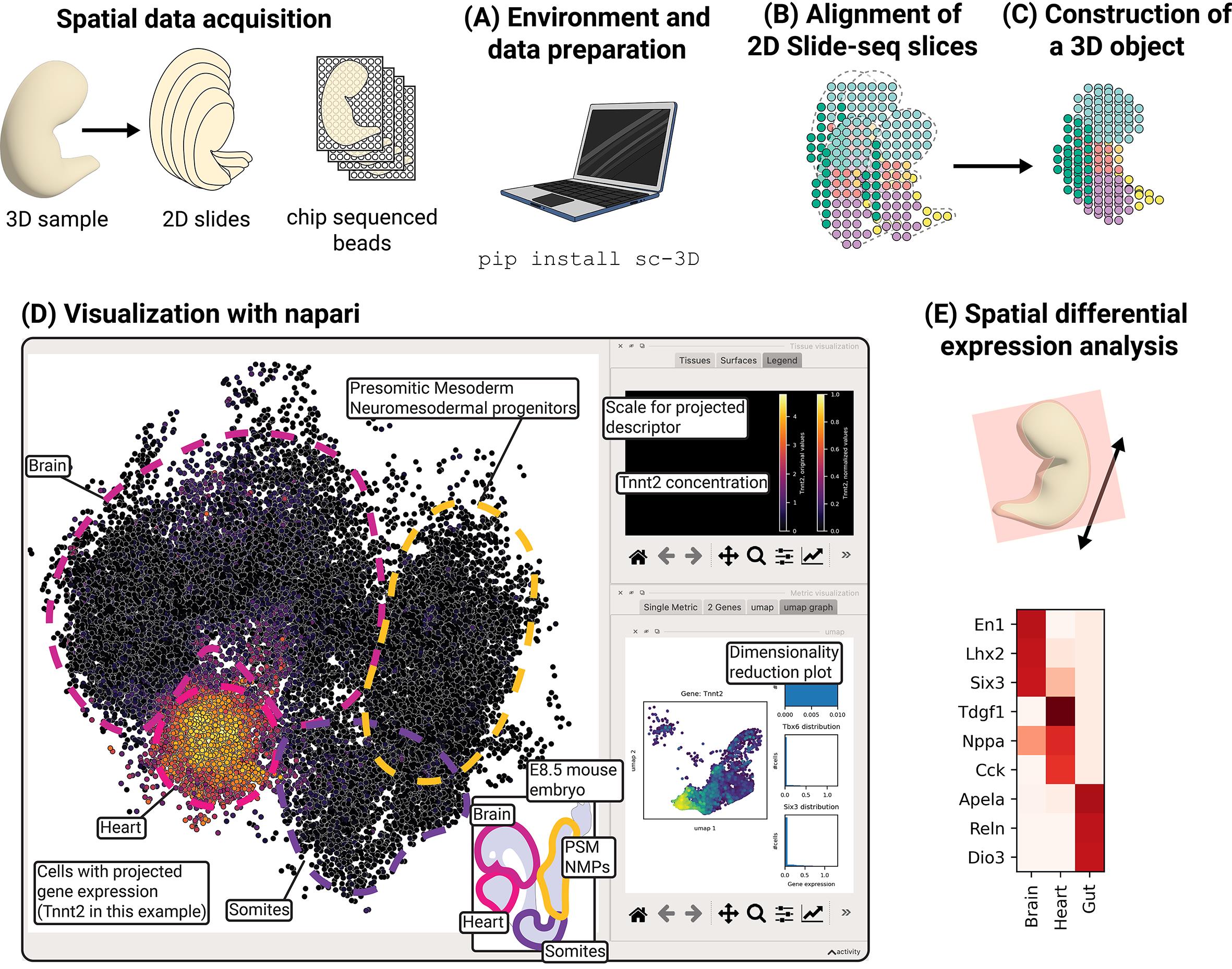
Reconstruction, visualization, and spatial differential expression analysis of 3D spatial transcriptomic data. The sc3D workflow comprises five stages: (A) environment setup and data preparation, (B) alignment of 2D Slide-seq slices, (C) construction of a 3D .sc3d object, (D) visualization with napari, and (E) spatial differential expression analysis.
Background
The way cells are positioned relative to each other influences how tissues function, guiding processes such as embryonic development, tissue repair, and disease progression. For example, during embryonic development, coordinated morphogenesis depends on precise spatial and temporal control of cell fate decisions, migration, and tissue interactions, giving rise to reproducible three-dimensional architectures from initially homogeneous progenitor fields [1–3]. Spatial omics technologies such as Slide-seq and Stereo-seq now enable genome-wide mapping of gene expression across serial two-dimensional sections, providing molecular insight into gradients, boundaries, and neighborhood interactions between cells. These approaches have revealed fine-grained transcriptional domains in development and disease [4–6]. Even though recent tools have started to provide means to analyze gene expression domains in 3D [7–9], spatial transcriptomics data remain inherently planar; each section captures only a local snapshot, and continuity across depth is lost. Consequently, the volumetric architecture of organs or complex systems (how domains connect, how gradients extend, and how cells interact in three dimensions) remains fragmented.
sc3D provides a computational framework to reconstruct three-dimensional spatial omics datasets from serial two-dimensional sections. The workflow estimates geometric transformations between adjacent slices, interpolates bead or spot coordinates along the z-axis, and merges them into a continuous volumetric dataset that preserves tissue geometry. Within this reconstructed volume, users can visualize gene expression distributions, quantify spatial gradients, and perform 3D-aware differential analyses to identify molecules enriched within defined regions or neighborhoods. The resulting registered .h5ad dataset can be explored interactively in the napari-sc3D-viewer, enabling virtual in situ hybridization, segmentation overlays, and volumetric quantification.
By providing an open-source, Python-based implementation integrated with the AnnData and Scanpy ecosystems [10], sc3D promotes reproducible, accessible 3D reconstruction and analysis across laboratories. Its design is modality-agnostic and generalizes to any spatial omics datasets that include x–y coordinates and slice identifiers, enabling quantitative 3D analysis across diverse samples. This integration opens the possibility to bridge spatial transcriptomics with other molecular modalities such as chromatin accessibility, DNA methylation, or spatial proteomics, which are now increasingly profiled in parallel. Together, these advances add another dimension to the quantification of tissue compartmentalization and morphogenetic coordination during embryogenesis [11], tumor progression [12], and regeneration [13].
Software and datasets
| Type | Software/dataset/resource | Version | Date | License | Access |
|---|---|---|---|---|---|
| Data | Mouse embryo Slide-seq E8.5. AnnData (.h5ad) with X_spatial, labels | 2023-04-05 | CC BY | free | |
| Data | Mouse embryo 1 Stereo-seq E16.5. AnnData (.h5ad) | 2022-05-12 | CC BY | free | |
| Software | sc3D (GitHub: GuignardLab/sc3D; PyPI: sc-3D) | 3.0.0 | 2025-06-17 | MIT | free |
| Software | napari-sc3D-viewer (GitHub: GuignardLab/napari-sc3D-viewer) | 2.0.0 | 2025-06-17 | MIT | free |
sc3D installation: The package supports Python ≥ 3.8 and is distributed on PyPI. We recommend creating a dedicated mamba/conda environment and installing sc3D via pip:
mamba create -n sc3d python=3.13mamba activate sc3dpip install sc-3DAlternatively, clone the repository (git clone https://github.com/GuignardLab/sc3D.git) and install in developer mode with pip install -e. For macOS machines with M1 chips, use miniforge to ensure compatibility.
Dependencies: sc3D depends on numpy, scipy, pandas, anndata, scanpy, matplotlib, and napari. Installing jupyter is recommended to run the example notebooks.
Data requirements: Input datasets must be stored as .h5ad anndata objects containing spatial coordinates and gene expression matrices. The x-y coordinates should be stored in obsm['X_spatial'], the array (slice) identifier in obs['orig.ident'], the tissue or cell cluster label in obs['predicted.id'], and gene names as indices or in var['feature_name'].
Slice ordering is inferred from the obs['orig.ident'] field by extracting numeric sequences from the identifier string using a regular expression. Specifically, sc3D identifies all contiguous numeric substrings separated by non-numeric characters and assigns the slice number based on the numeric sequence at position array_id_num_pos. By default (array_id_num_pos = -1), the last numeric sequence in the identifier is used.
For example, identifiers such as coverslip_03, sliceA5, or E8p5_slice_012 yield numeric sequences 03, 5, and 8, 5, 12, respectively. With the default setting, these would be interpreted as slice numbers 3, 5, and 12. If a different numeric component should define slice order, users can specify the appropriate index via the array_id_num_pos parameter.
These column name and parsing behaviors can be customized via the parameters tissue_id, array_id, pos_id, gene_name_id and pos_reg_id. Example of unregistered datasets [14] are available from Figshare ( https://figshare.com/s/9c73df7fd39e3ca5422d).
Output formats: The workflow produces registered .h5ad files containing 3D coordinates and interpolation layers, .sc3d objects used by sc3D-viewer, and optional .h5ad files representing extracted slices or downsampled datasets. The napari-sc3D-viewer plugin (installed via pip install napari-sc3D-viewer) loads these files for interactive exploration.
Hardware requirements and alternatives
sc3D is fully CPU-based and does not require GPU acceleration. For large datasets (for example, on the order of ~500,000 beads), ≥16 GB of RAM is recommended to perform registration and interpolation without downsampling; however, smaller memory configurations can still be used by downsampling the dataset or by limiting interpolation and visualization steps. While this protocol was tested on a local workstation (macOS system, 10-core CPU, 32 GB RAM), sc3D relies exclusively on standard Python scientific libraries and can be executed without modification on cloud or high-memory compute nodes. Detailed tested hardware and software specifications are provided in the reproducibility note.
Procedure
A Jupyter notebook accompanies this protocol as Supplementary Material (Code S1). It contains all commands, parameters, and example outputs described below, pre-configured for a test dataset. Users can run the notebook directly to reproduce each step from slice registration to 3D visualization and spatial differential expression. The notebook is designed to serve both as a tutorial and a template for adapting the workflow to new Slide-seq datasets.
A. Environment setup and data preparation
1. Create a fresh virtual environment. Use mamba (faster conda), conda, or venv to isolate dependencies. For example, run:
mamba create -n sc3d -y python=3.132. Activate it and install sc3D, which will also install its dependencies automatically:
mamba activate sc3dpip install sc-3DIf necessary, install pip before:
mamba install pip3. Prepare the input data. Download the unregistered .h5ad file of our Slide-seq dataset from figshare ( https://figshare.com/s/9c73df7fd39e3ca5422d) or your own experiment. If you use your own data, ensure that spatial coordinates are stored in obsm['X_spatial'], slice identifiers in obs['orig.ident'], and tissue labels in obs['predicted.id']. If the dataset uses different column names, specify them in the SpatialOmicArray constructor via array_id, tissue_id, etc. (see section B).
4. Install optional tools (not required for building the sc-3D but useful for visualization). Install jupyter (mamba install jupyter). You can also download the pre-made example notebooks from the sc3D repository (github.com/GuignardLab/sc3D/tree/main /notebooks) to familiarize yourself with the workflow:
mamba install jupyter5. You can start the notebook and import the necessary libraries for section B (start of notebook Code S1).
import jsonfrom matplotlib import pyplot as pltimport numpy as npfrom sc3D import SpatialOmicArray%matplotlib inlineB. Alignment of 2D Slide-seq slices
This stage registers consecutive slices and produces a unified 3D point cloud. Expected time is ~30–90 min per atlas, depending on size and hardware.
1. Specify parameters. sc3D requires several user-defined parameters that control slice alignment, outlier removal, and interpolation along the reconstruction axis. The values for th_d, outlier_threshold, and nb_interp used in this protocol were selected empirically based on the physical properties of the Slide-seq mouse embryo datasets analyzed in the original study. Specifically, th_d = 150 μm reflects the expected maximum spatial displacement between corresponding beads in adjacent sections given typical slice spacing (50–80 μm) and moderate tissue deformation. The outlier_threshold = 0.6 was chosen to remove spatially isolated beads while preserving coherent tissue regions, and nb_interp = 5 was selected to balance smooth interpolation of the 3D volume with computational efficiency. These values should be interpreted as practical starting points rather than optimized defaults. For other datasets, parameters should be adapted based on spatial resolution, bead density, slice spacing, and the expected magnitude of tissue deformation. Recommended values and adjustment guidelines are summarized in Table 1.
Table 1. Alignment parameters
| Parameter | Purpose | Value used in this protocol | Small datasets (<50k beads) | Medium datasets (50k–250k beads) | Large datasets (>250k beads) | Notes and tuning guidelines |
| th_d (μm) | Maximum allowed distance between matched beads in adjacent slices during registration | 150 | 80–120 | 120–200 | 150–250 | Increase with larger slice spacing or stronger tissue deformation; decrease to prevent spurious matches in dense datasets |
| outlier_threshold | Posterior-probability threshold (Gaussian mixture model on nearest-neighbor distances) used to filter spatially isolated beads | 0.6 | 0.4–0.6 | 0.5–0.7 | 0.6–0.8 | Higher values remove more isolated beads; overly aggressive filtering may remove true tissue regions |
| nb_interp | Number of interpolated layers inserted between consecutive slices | 5 | 3–5 | 5–7 | 3–5 | Higher values yield smoother volumes but increase memory usage; reduce for very large datasets |
| xy_resolution (μm) | Physical spatial resolution in the x–y plane | Dataset-specific (e.g., 0.6 for Slide-seq) | Assay-dependent | Assay-dependent | Assay-dependent | Must match the physical resolution of the spatial transcriptomics platform |
| array_id_num_pos | Position of numeric token used to infer slice order from obs['orig.ident'] | −1 (last numeric group) | −1 | −1 | −1 | Change only if slice identifiers contain multiple numeric groups |
| tissue_weight | Optional weighting of selected tissue labels during registration | None (example provided) | None | Optional | Optional | Use only to stabilize alignment by anchoring large, continuous tissues |
As a general rule, th_d should scale with slice spacing and expected tissue distortion, whereas xy_resolution must always reflect the physical resolution of the assay. Users are encouraged to inspect registration QC plots after alignment and adjust parameters iteratively if tissues appear fragmented, over-warped, or discontinuous across slices.
# Required files# input AnnData with X_spatial and labelsdata_path = "data/E8.5.h5ad"# Path to the output folderoutput_folder = "out/"# (optional) mapping of tissue ids to names, find an example in github.com/GuignardLab/sc3D/tree/main/datacorres_tissues = "data/corresptissues.json"# list of tissue ids to ignore during registrationtissues_to_ignore = [13, 15, 16, 22, 27, 29, 32, 36, 40, 41]# Gives more weight to some tissues to help the alignmenttissue_weight = {21: 2000, 18: 2000}Note: The tissue_weight parameter is an optional heuristic that can be used to stabilize slice alignment by increasing the influence of selected tissue labels during the registration optimization. In practice, higher weights are assigned to large, spatially continuous tissues that are expected to be present across many consecutive sections (for example, neural tube or mesodermal compartments in embryos). The specific values shown here are provided as an example and were chosen empirically to emphasize these reference tissues in the mouse embryo dataset; they do not represent universal or optimized defaults. For new datasets, tissue weighting can be omitted or adjusted based on tissue size, continuity, and annotation confidence.
# Visualization palette (optional)with open("data/tissuescolor.json") as f: colors_paper = {eval(k): v for k, v in json.load(f).items()}# Registration / interpolation parametersxy_resolution = 0.6 # μm per bead; set to your Slide-seq resolution# for QC plots/interpolation# list of marker genes to visualize and monitor during registration.genes_of_interest = ["Sox2","Shh","Pax3","Mesp2","Myf5"]nb_CS_begin_ignore = 0 # number of slices to ignore at the beginningnb_CS_end_ignore = 4 # number of slices to ignore at the end# Distance max that two beads can be linked together between slicesth_d = 150 # in μm# Threshold below which the beads will be considered noise.# Value between 0 (all beads taken) and 1 (almost no beads taken)outlier_threshold = 0.6# Number of interpolated layers between two consecutive slicesnb_interp = 52. Initialize the SpatialOmicArray object in the same Python session or notebook where you already imported the SpatialOmicArray class:
spatialsample = SpatialOmicArray( data_path, tissues_to_ignore, corres_tissues, tissue_weight=tissue_weight, xy_resolution=xy_resolution, genes_of_interest=genes_of_interest, nb_CS_begin_ignore=nb_CS_begin_ignore, nb_CS_end_ignore=nb_CS_end_ignore, store_anndata=True )3. Critical step: Verify slice order before proceeding.
As stated in the data requirement section, sc3D infers the relative order of tissue sections automatically from the slice identifiers stored in adata.obs['orig.ident']. All numeric substrings present in this field are extracted, and the numeric value at position array_id_num_pos (by default, the last numeric group) is used to define slice order along the reconstruction axis.
Before running the 3D registration, users must verify that the inferred slice order matches the biological ordering of sections (e.g., anterior–posterior or proximal–distal). This can be done by printing the sorted slice identifiers and visually confirming that consecutive sections correspond to neighboring anatomical regions.
print(sorted(spatialsample.anndata.obs["orig.ident"].unique()))If the inferred order is incorrect, users should either rename slice identifiers in obs['orig.ident'] or adjust the array_id_num_pos parameter so that the correct numeric group is used for ordering. Incorrect slice ordering will propagate through the entire reconstruction and lead to biologically implausible 3D structures.
4. Critical step: Remove spatial outliers. Call spatialsample.removing_spatial_outliers to discard beads with anomalous spacing. A value of 0.6 retains most beads; increase it to remove more noise. Inspect scatter plots of beads colored by tissue to ensure that true structures remain intact (Figure 1, see Code S1). Users should visually inspect the spatial distribution of retained and removed beads after this step to ensure that coherent tissue regions are preserved and that biologically meaningful structures are not inadvertently discarded. Overly aggressive filtering may lead to tissue fragmentation and impaired registration.
spatialsample.removing_spatial_outliers(th=outlier_threshold)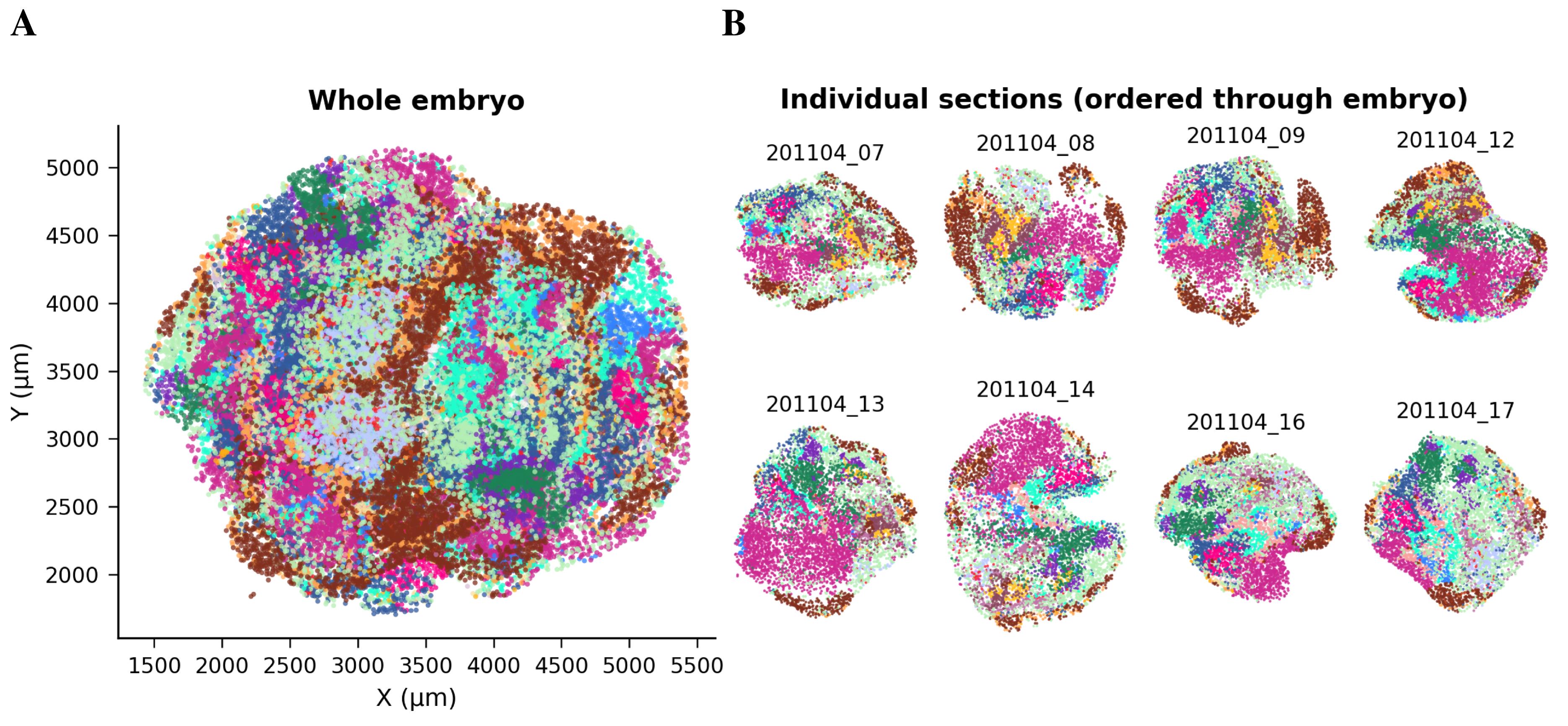
Figure 1. Spatial distribution of beads in Slide-seq slides before registration. (A) Overview of the complete dataset showing all Slide-seq slides, with beads colored by tissue identity (obs[‘predicted.id’]) prior to 3D alignment. Axes correspond to raw spatial bead coordinates (μm). (B) Representative individual slices sampled evenly along the embryo sequence (obs[‘orig.ident’]). Each subplot shows the original 2D spatial organization within a single slide. These quality-control plots, generated after outlier removal (spatialsample.removing_spatial_outliers), assess if tissue domains are intact before registration and interpolation.
5. Perform 3D registration. Execute spatialsample.registration_3d to align consecutive slices. The method employs tissue-weighted optimal transport to link beads between slices and B-spline interpolation to compute intermediate layers. The number of interpolated layers is set by nb_interp; thresholds and other parameters are as defined above. Registration time scales with the number of beads and slices; 13 slices with ~200,000 beads take ~30 min on a 16-core workstation (see https://github.com/GuignardLab/sc3D/blob/main/txt/scSpatial.pdf).
spatialsample.registration_3d()Note: Output attributes (sc3D internal representation). In SpatialOmicArray, all_cells stores the internal indices of the beads/spots currently included in the analysis (initialized as 0..N−1 when loading the AnnData object and updated after filtering steps such as spatial outlier removal). tissue is a dictionary mapping each bead/spot index to its tissue or cluster label derived from adata.obs[tissue_id]. After registration, final contains the registered 2D (x,y) coordinates for each bead/spot following sequential slice alignment. The corresponding 3D registered coordinates are stored in pos_3D, which combines the final with the slice’s z_pos.
6. Pause point: Before downstream analysis, users should verify that the reconstructed slices are anatomically plausible. This includes checking continuity of major tissues across adjacent sections, absence of abrupt rotations or flips, and consistency with known anatomical landmarks. If misalignments are observed, registration parameters should be adjusted and the alignment rerun. Then, save the registered dataset. After registration completes, save the result to an .h5ad file using spatialsample.save_anndata. This file contains 3D coordinates in obsm['X_spatial_registered'] and can be opened by sc3D-viewer.
spatialsample.save_anndata(output_folder + "/E8.5_registered.h5ad")# or replace E8.5 by the name of your fileC. Construction of the 3D .sc3d object
This stage interpolates intermediate layers, generates a dense 3D grid, and prepares the data for visualization and downstream analyses.
1. Reconstruct intermediate layers. From the registered SpatialOmicArray object, call
spatialsample.reconstruct_intermediate(th_d=th_d, genes=genes_of_interest)This function interpolates expression values and positions along the z-axis, creating a continuous 3D representation. It also updates spatialsample.final with the registered coordinates.
2. For datasets exceeding 500,000 beads, use spatialsample.downsample(spacing=...) to aggregate beads on a regular 2D grid slice-by-slice, where spacing is the grid step (in the same units as your coordinates, typically μm). For each grid point, expression values are the mean of beads within radius spacing/2, and the tissue label is the majority class in that neighborhood. The function returns a new AnnData object. Downsampling reduces memory requirements at the expense of resolution.
spatialsample.downsample(spacing=10)3. Extract and visualize slices. Use spatialsample.plot_slice to visualize cross-sections at arbitrary orientations (Figure 2). angles is a 3-element vector defining rotations around the x-, y-, and z-axes; origin is a 3D coordinate selecting the center of the slice; thickness controls the slice depth; and tissues restricts the plot to selected tissues. To examine gene expression, set gene='T' or a list of two genes and adjust the main_bi_color parameter to choose color pairs. Figures are saved to PDF via output_path. A working example:
# Compute the 3D centroid of selected tissuesselected_tissues = {30, 31}coords = np.array([ spatialsample.final[c] for c in spatialsample.all_cells if spatialsample.tissue[c] in selected_tissues])origin = np.hstack([coords.mean(axis=0), 80]) # shift 80 μm upward in z# Slice orientation (rotations around x, y, z axes, in degrees)angles = np.array([-5.0, 5.0, 0.0])# Plot virtual slice using sc3D's native methodpoints = spatialsample.plot_slice( angle=angles, color_map=colors_paper, origin=origin, thickness=30, tissues=[18, 30, 31], nb_interp=5,)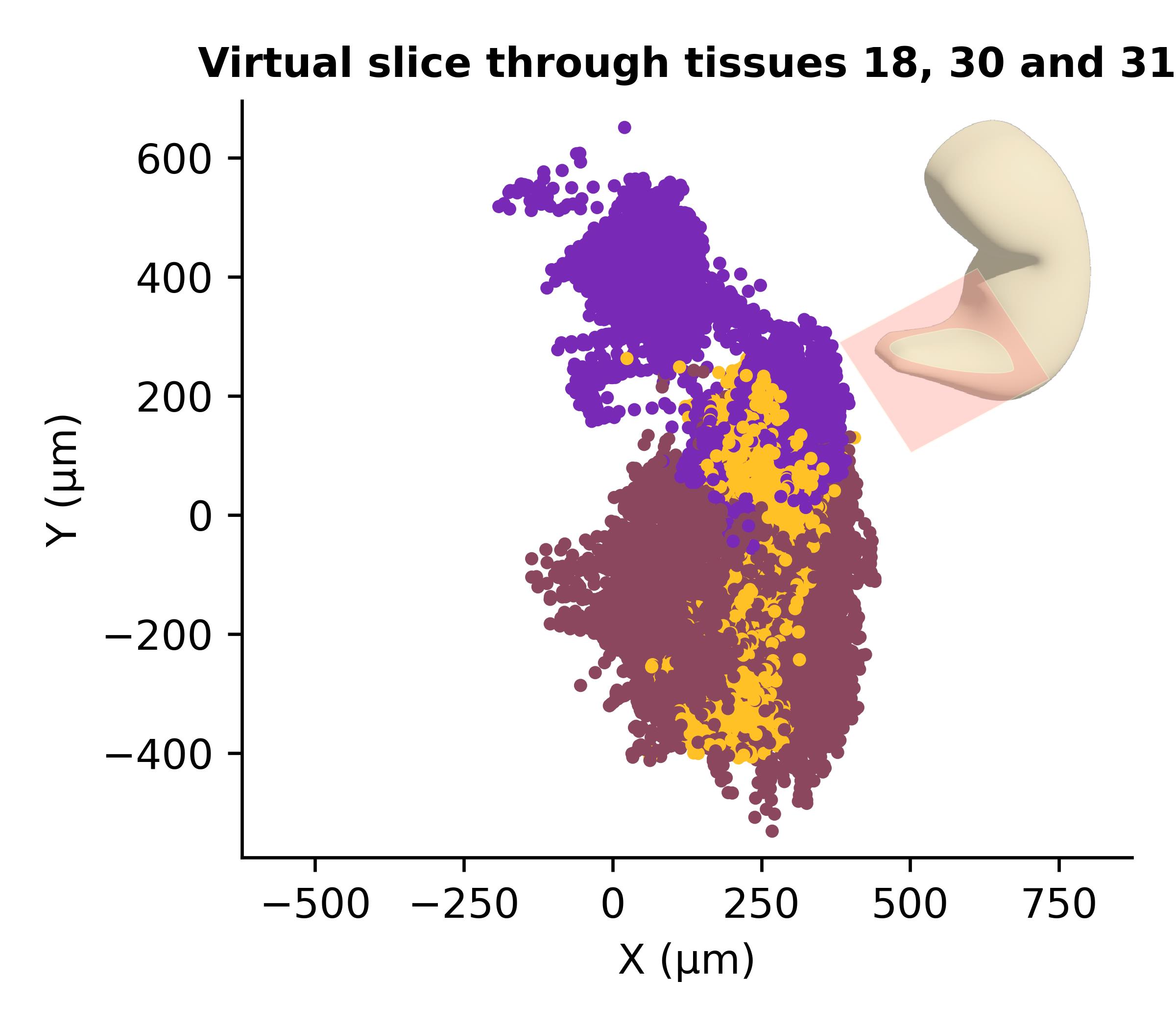
Figure 2. Virtual slicing of the reconstructed spatial sample. A virtual cross-section through the reconstructed 3D sample showing the spatial distribution of tissues 18, 30, and 31 (somites, presomitic mesoderm, and neuromesodermal progenitors). The slice was positioned at the centroid of tissues 30–31 and tilted by (-5°, +5°, 0°) along the x, y, and z axes, respectively, with a thickness of 30 μm. Each point represents an individual Slide-seq bead colored by tissue identity. The inset illustrates the approximate position and orientation of the virtual slice within the 3D volume.
4. Once inspection of slices is completed, we can proceed to generate a sc3d file. Save the fully reconstructed dataset as an anndata file or a custom .sc3d object using spatialsample.save_anndata. A sc3d file is simply an anndata object with registered coordinates and metadata; the extension facilitates recognition by the napari plugin. Additional functions spatialsample.anndata_slice() and spatialsample.anndata_no_extra() allow the extraction of arbitrary slices with or without interpolation (see documentation of the library or github.com/GuignardLab/sc3D).
spatialsample.save_anndata('out/E8.5_reconstructed.h5ad')D. Visualization using napari-sc3D-viewer
1. Open the terminal in the same environment you created before for sc3D. Install napari and our plugin napari-sc3D-viewer. Then, launch napari by executing it from the command line. If you run into issues installing napari, visit https://napari.org/stable/tutorials/fundamentals/installation.html for more detailed instructions and troubleshooting.
python -m pip install "napari[all]"
pip install napari-sc3d-viewer
napari
Note: You can also install the viewer directly from within Napari via Plugins → Install/Uninstall Plugins → Search “napari-sc3D-viewer.” This method automatically installs both napari-sc3D-viewer and sc3D.
2. Load the .sc3d file. In napari, choose Load spatial single cell from the Plugins > napari-sc3D-viewer menu and select the reconstructed.h5ad file (Figure 3). The expected dataset is a scanpy/anndata h5ad file together with an optional json file that maps cluster id numbers to actual tissue/cluster names. The json file should look like the following:
{ "1": "Endoderm", "2": "Heart", "10": "Anterior neuroectoderm"}Note: If no json file or a wrong json file is given, the original cluster id numbers are used.
3. The viewer is expecting four different columns to be present in the h5ad file:
• The cluster id column (by default named “predicted.id” that can be accessed as data.obs['predicted.id']).
• The 3D position column (by default named “X_spatial_registered” that can be accessed as data.obsm['X_spatial_registered']).
• The gene names, if not already in the column name (by default named “feature_name” that can be accessed as data.var['feature_name']).
• umap coordinates (by default named “X_umap” that can be accessed as data.obsm['X_umap']).
• If the default column names are not consistent with your dataset, they can be changed in the tab Parameters (see button 3 in Figure 3) next to the tab Loading files.
Note: The input AnnData object must contain a precomputed UMAP embedding stored in obsm['X_umap']. This embedding is not computed by sc3D and should be generated upstream (for example, using Scanpy) prior to visualization.
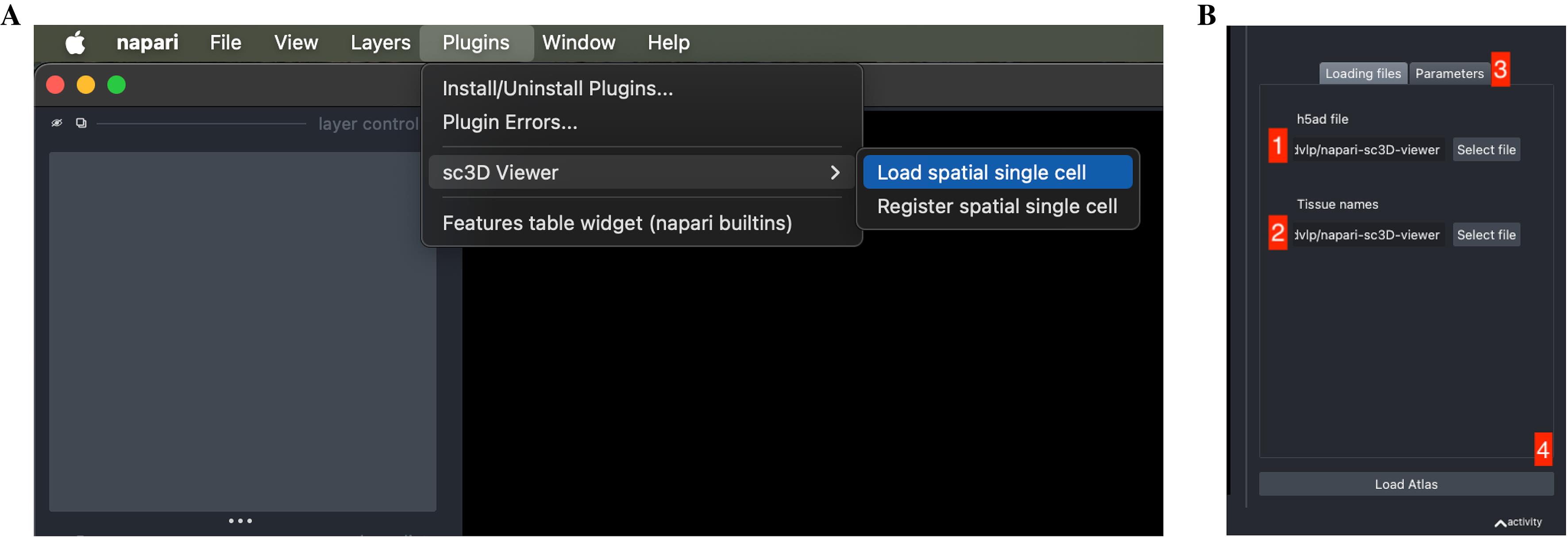
Figure 3. Loading a reconstructed spatial experiment into napari-sc3D-viewer. (A) Launching the sc3D Viewer plugin from the Plugins menu in Napari. Select Load spatial single cell to open the viewer interface. (B) The loading panel of napari-sc3D-viewer. The user must (1) provide the path to the .h5ad file containing the reconstructed embryo and (2) the optional tissue correspondence file, and (3) verify or adjust the expected column names in the Parameters tab. Once all fields are correctly set, pressing Load Atlas (4) loads the dataset into the 3D viewer.
4. Once all the data paths and fields are correctly informed, pressing the Load Atlas button (see button 4 in Figure 3) will load the dataset. The viewer displays the 3D point cloud with default tissue colors. Use the interactive controls to rotate, zoom, and clip the dataset.
5. Explore gene expression. The sc3D-viewer panel allows selection of genes for virtual in situ hybridization (vISH). Enter a gene name or choose two genes for bi-color overlays (Figure 4). Adjust the intensity scale to highlight gradients. Annotated tissues can be toggled on or off to focus on specific structures.
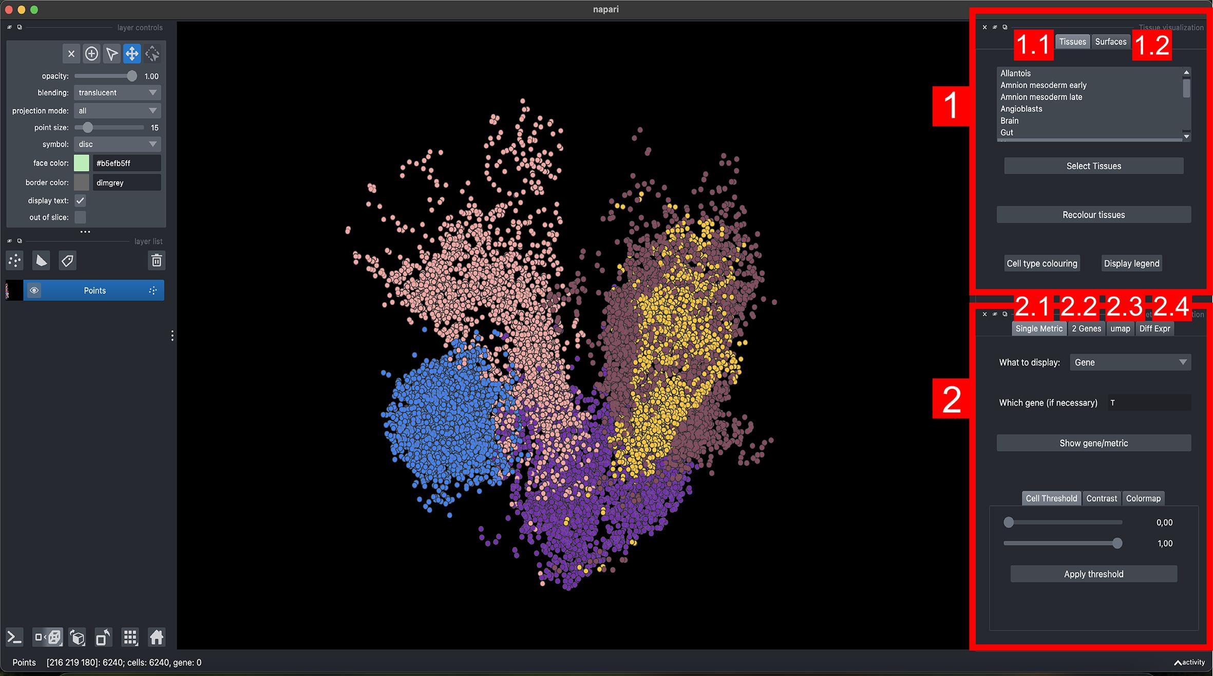
Figure 4. Interface of napari-sc3D-viewer for tissue and gene visualization. The viewer is organized into two main panels: (1) Tissue visualization and (2) Metric visualization, each containing several interactive tabs for different modes of exploration. (1.1) Tissues tab: displays individual tissues and allows selection, recoloring, and legend visualization of tissue identities. (1.2) Surfaces tab: generates and renders coarse 3D tissue surfaces for spatial context. (2.1) Single metric tab: visualizes single-gene expression or any numerical metric embedded in the dataset, with controls for contrast, colormap, and thresholding. (2.2) Two-genes tab: displays co-expression patterns between pairs of genes. (2.3) UMAP tab: shows the UMAP projection of selected cells and allows manual sub-selection of clusters for focused visualization. (2.4) Differential expression tab: identifies and plots genes differentially expressed across selected tissues or clusters.
6. Select the Diff Expr tab in the Metric visualization panel, choose a tissue (e.g., Heart), and click Display differentially expressed. The top differentially expressed genes will appear in a dropdown menu. Selecting a gene (e.g., Nppa) displays its spatial expression pattern across the embryo, highlighting regions of enrichment (Figure 5).
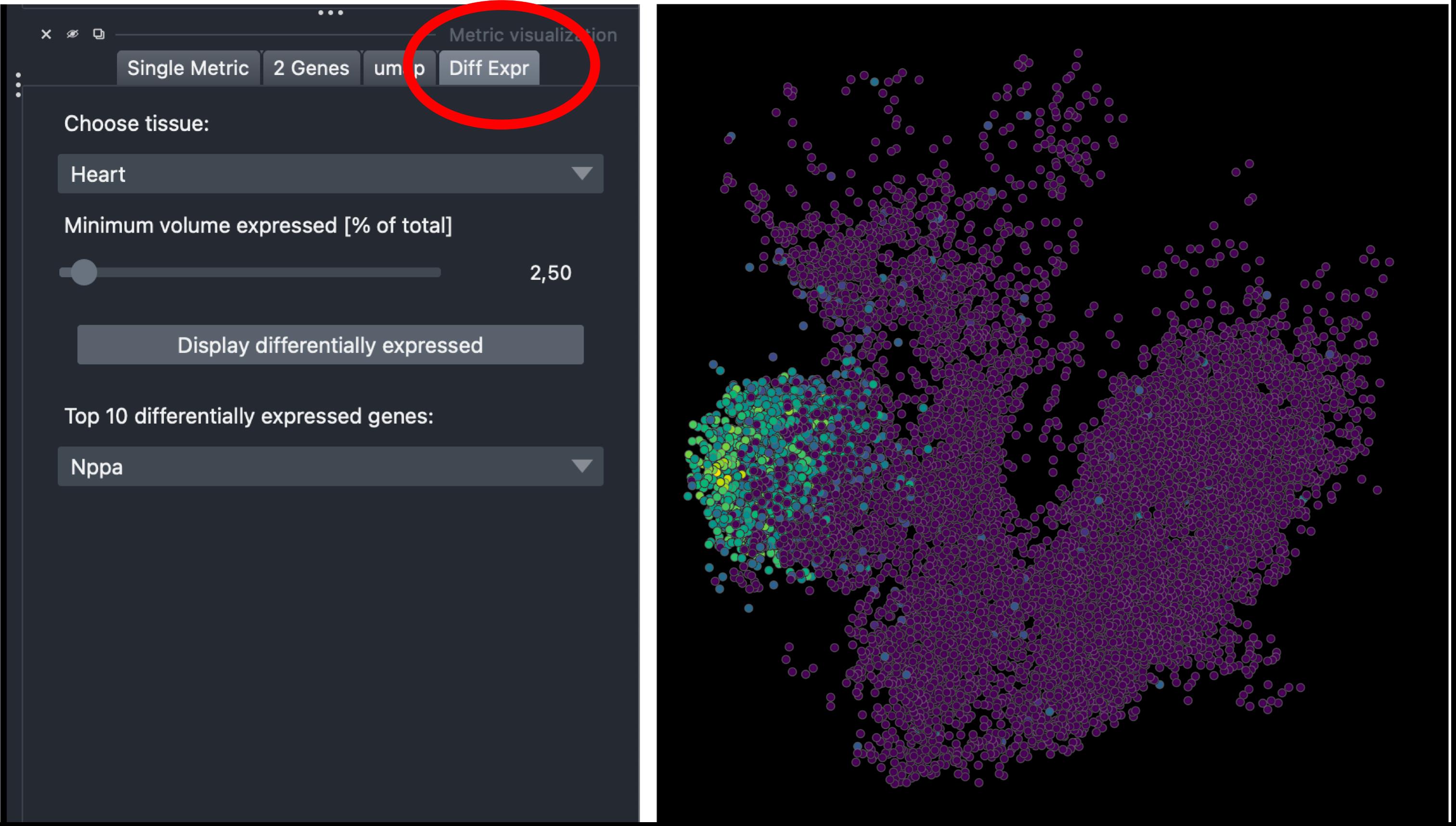
Figure 5. Differential expression visualization in napari-sc3D-viewer. Spatial expression of Nppa in the reconstructed embryo, obtained by selecting Heart in the Diff Expr tab (left panel, circled in red). Points are colored by expression intensity using viridis colormap, revealing localized enrichment in the heart region (right panel).
7. Select spatial regions directly from the UMAP view. Open the UMAP tab in the Metric visualization panel and click UMAP graph to display the low-dimensional embedding of all beads. Using the selection tool, draw directly on the UMAP to highlight specific clusters or regions. The selected beads will automatically be displayed in 3D on the embryo view, enabling interactive linking between transcriptomic and spatial domains (Figure 6).
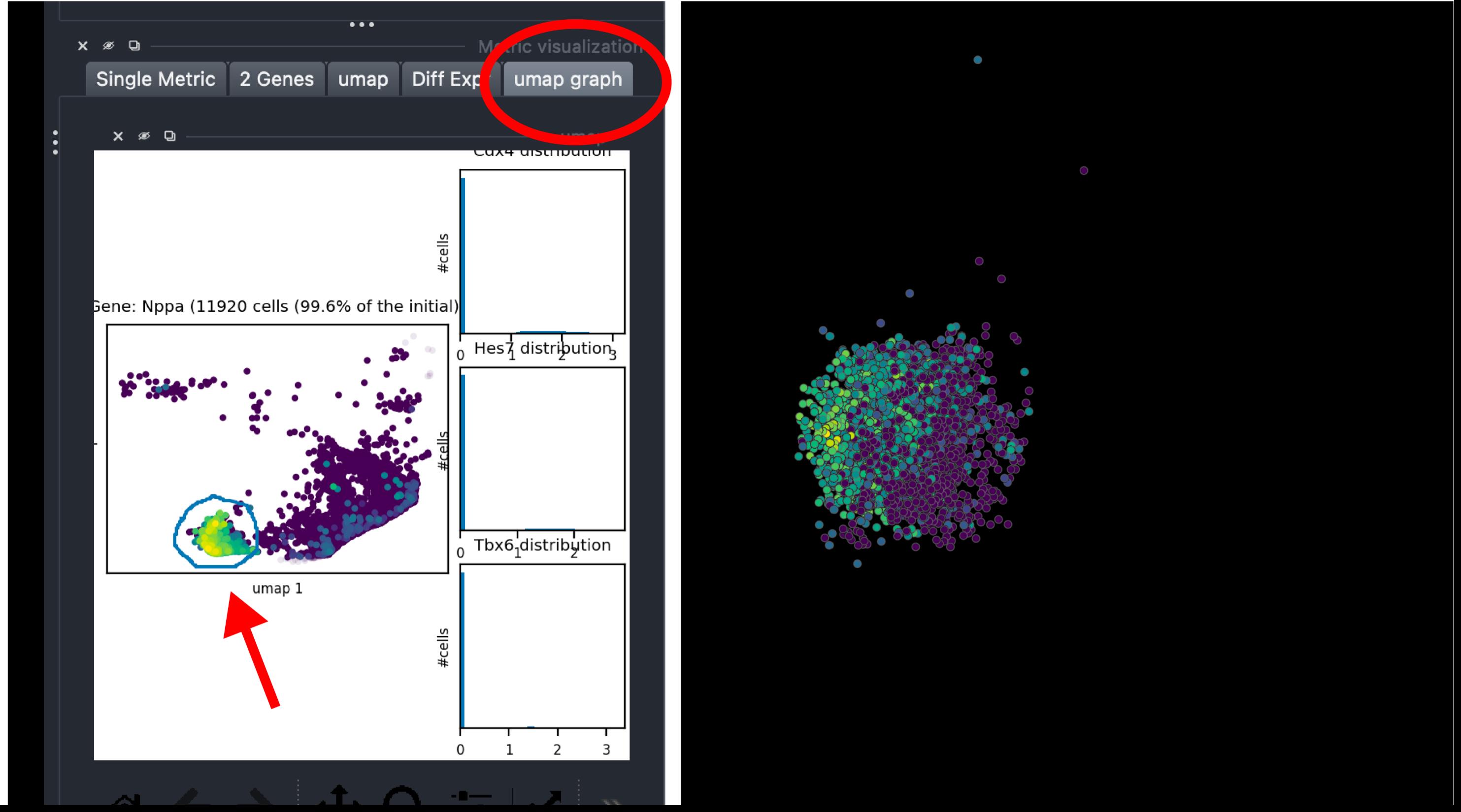
Figure 6. Interactive UMAP-based selection in napari-sc3D-viewer. The UMAP graph view allows manual selection of specific bead clusters (red arrow, left) based on their transcriptomic similarity. The corresponding cells are simultaneously highlighted in the 3D embryo view (right), enabling intuitive spatial inspection of selected populations.
8. Visualize the co-expression of two genes. Select the 2 Genes tab in the Metric visualization panel to display the spatial co-expression of two genes. Enter the main gene (e.g., Nppa) and a secondary gene (e.g., Tnnt2), then adjust the Low and High threshold sliders to refine expression ranges. Click Map Colors to render the two expression domains simultaneously in 3D, with each gene assigned a distinct color (Figure 7).
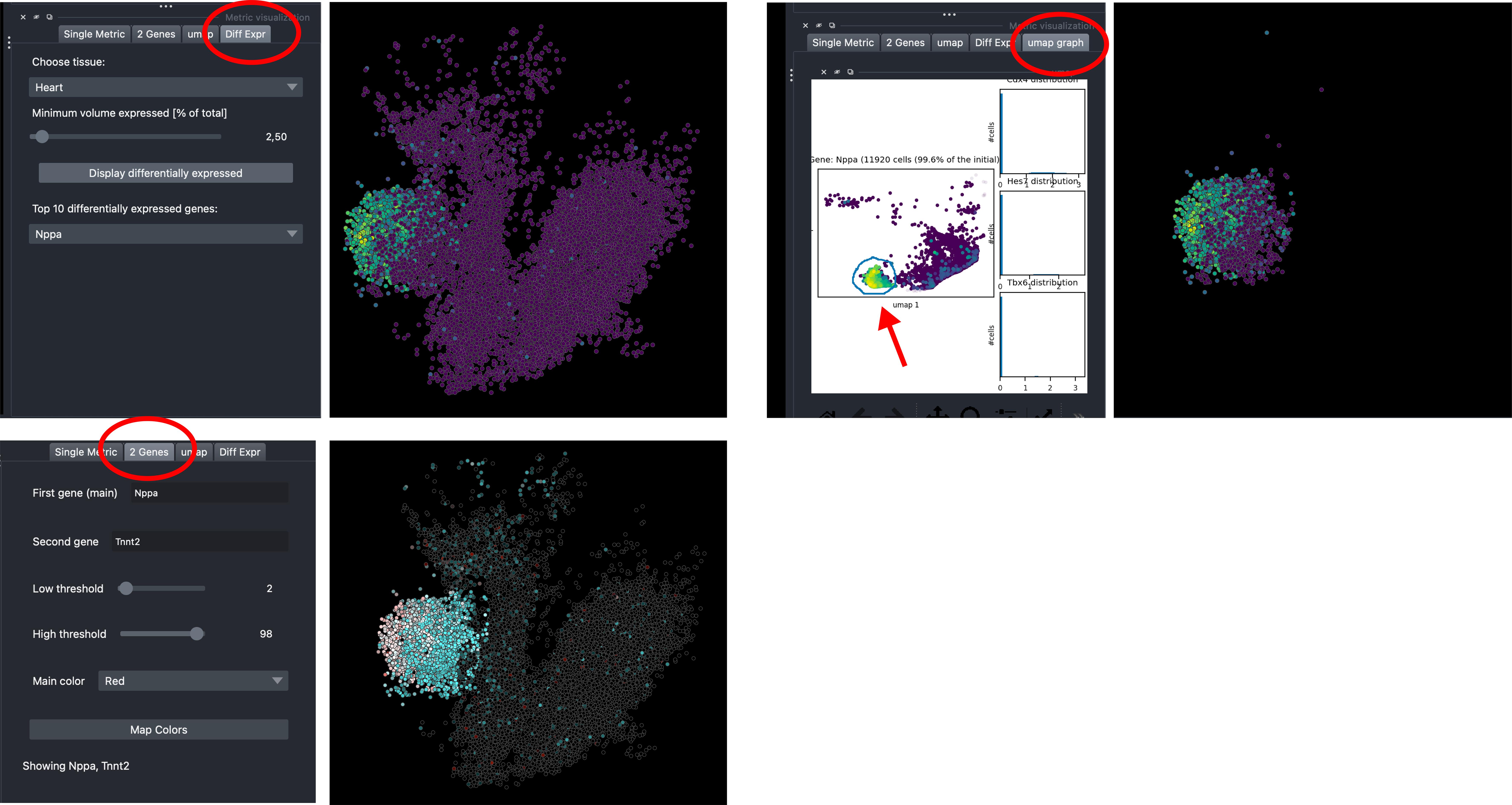
Figure 7. Co-expression analysis in napari-sc3D-viewer. The 2 Genes tab (left panel, circled in red) enables simultaneous visualization of two genes across the reconstructed embryo. Here, Nppa (red) and Tnnt2 (cyan) expression patterns are displayed (right panel), illustrating complementary or overlapping spatial domains within the same 3D view.
9. Export figures. Use the screenshot tool or napari’s built-in exporter to save images or videos of the embryo in different orientations. For publication-quality figures, adjust point size, color maps, and opacity.
E. Spatial differential gene expression analysis in Python (sc3D library)
All analyses demonstrated in the napari-sc3D-viewer (Section D) can also be run programmatically using the sc3D Python library, along with extended quantifications. This enables customized plotting, refined quantification, and automated workflows.
1. If you are starting a new session, re-load the sc3D library and the reconstructed embryo saved in section C. Then, define the list tissues_to_process (e.g., [21, 30, 31]) and a volume threshold th_vol (e.g., 0.025):
from sc3D import SpatialOmicArray
spatialsample = SpatialOmicArray( 'out/E8.5_reconstructed.h5ad', corres_tissues='data/corresptissues.json', store_anndata=True)tissues_to_process = [21] #[5, 10, 12, 18, 21, 24, 30, 31, 33, 34, 39]th_vol = .025 # minimum volume fraction to take into account a geneNote: Setting th_vol to 0 will consider all genes. This is not recommended since it will consider a lot of genes that are either not expressed at all or genes that are expressed everywhere.
2. Compute spatial differential expression. Run get_3D_differential_expression() to identify genes enriched within each selected tissue compared with the rest of the embryo. The first call computes global statistics and may take several minutes depending on dataset size; subsequent calls reuse shared quantities.
_ = spatialsample.get_3D_differential_expression(tissues_to_process, th_vol, all_genes=False)If we want to add a tissue to the set of tissues already treated, it can be done easily and will be much faster since all the pre-processing is stored:
_ = spatialsample.get_3D_differential_expression([7, 24], th_vol, all_genes=False);3. Visualize top spatial markers (Figure 8A). Plot the top differentially expressed genes using:
spatialsample.plot_top_3D_diff_expr_genes([7, 21, 24], nb_genes=3)Note that not all tissues have to be plotted. Also, if a tissue asked for has not already been computed, the function informs the user about it. Set nb_genes to display only the top n genes per tissue. Setting repetition_allowed=True allows the same gene to appear in multiple tissues. compute_z_score controls whether raw values or z-scores are plotted.
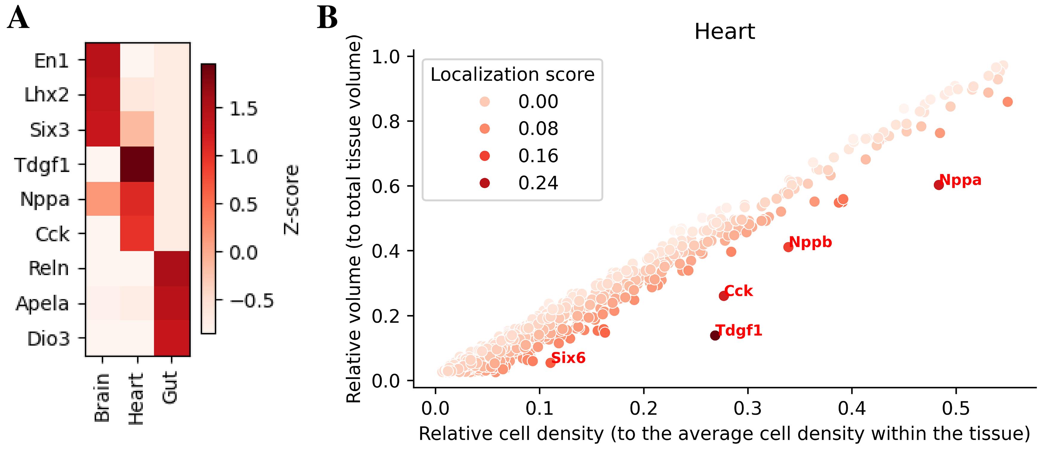
Figure 8. Spatially enriched genes and volume–density relationship. (A) Top differentially expressed genes across brain, heart, and gut. (B) In the heart, relative volume and cell density highlight highly localized genes (Nppa, Nppb, Cck, Tdgf1).
4. Inspect volume–density distributions (Figure 8). Call spatialsample.plot_volume_vs_neighbs to visualize the relative volume occupied by expressing cells vs. their density for a given tissue. Optional arguments print_genes or print_top annotate specific genes.
spatialsample.plot_volume_vs_neighbs(21, print_top=5, palette='Reds')To quantify spatial localization of gene expression within each tissue, we can summarize for every gene two statistics: (i) the fraction of tissue volume occupied by expressing beads (“relative volume”), and (ii) the local density of expressing beads, measured as the average number of expressing neighbors normalized to the tissue-wide average (“relative cell density”). For genes that are broadly distributed within a tissue, these two quantities follow an approximately linear relationship: genes that cover a larger fraction of the tissue tend to display lower local density, whereas genes with more restricted expression usually maintain similar or higher local density in a smaller volume [14]. Thus, we can fit a linear regression of relative volume as a function of relative density and define a localization score as the vertical residual from this regression. Genes with high localization scores occupy less tissue volume than expected for their density and are therefore inferred to be spatially localized (Figure 8B).
5. Export results. The differential expression table is stored in spatialsample.diff_expr and can be exported as a pandas DataFrame. Use spatialsample.print_diff_expr_genes to print the top markers.
spatialsample.print_diff_expr_genes(21, nb=10)Table 2 includes per-gene localization scores, density metrics, and relative expression volumes, allowing integration with downstream statistical analyses.
Table 2. Top spatially enriched genes identified by sc3D differential expression analysis
| Gene name | Volume ratio | Avg.# neighbors ratio | Localization score | Gene row ID |
|---|---|---|---|---|
| Tdgfl | 0.138456 | 0.268130 | 0.311707 | 2152 |
| Nppa | 0.605553 | 0.483951 | 0.214192 | 1519 |
| Cck | 0.260555 | 0.277083 | 0.204938 | 359 |
| Nppb | 0.411183 | 0.337637 | 0.158007 | 1520 |
| Six6 | 0.054013 | 0.109274 | 0.124117 | 1966 |
| Vsnl1 | 0.147204 | 0.163287 | 0.123420 | 2306 |
| Hba-x | 0.550019 | 0.392224 | 0.112648 | 1073 |
| Nr2f1 | 0.157855 | 0.162024 | 0.110607 | 1525 |
| Cited1 | 0.153290 | 0.157363 | 0.107188 | 426 |
| Hbb-bh1 | 0.548498 | 0.387230 | 0.105617 | 1074 |
Validation of protocol
This protocol has been used and validated in the following research article(s):
• Kumar et al. [14]. Spatiotemporal transcriptomic maps of whole mouse embryos at the onset of organogenesis. Nature Genetics. (Figures 1 and 3a–b).
The sc3D workflow was validated using serial Slide-seq datasets of mouse embryos at embryonic days (E) 8.5–9.0 [14]. After registration, the reconstructed virtual embryos reproduced major anatomical structures (including the heart tube, neural tube, somites, and brain) and allowed quantitative measurement of tissue volumes across replicates. Increasing the distance between sections produced minimal distortion of rotation axes, demonstrating robustness to reduced sampling. In total, ~27,000 genes were mapped onto the digital embryos, enabling virtual in situ hybridization and the calculation of localization scores. This analysis identified regionally enriched genes such as Nppa, Tdgf1, and Sfrp5 in the developing heart and Foxg1, Barhl2, and En1 in the brain. Comparisons with PASTE [15] showed that sc3D achieved higher registration accuracy with shorter computation time, while PASTE required less parameter tuning and may therefore be more straightforward for exploratory analyses. In the original study [14], this benchmarking was performed using Slide-seq v2 data from mouse E8.5–E9.0 embryos, as well as 10x Genomics Visium data from the human dorsolateral prefrontal cortex (DLPFC), where sc3D was compared with PASTE. Registration accuracy was evaluated using multiple complementary quantitative approaches ([14], Extended Data Figure 4), including (i) bead-to-bead tissue concordance metrics across adjacent sections, (ii) robustness analyses assessing sensitivity to increasing inter-slice distances and perturbations of the reconstruction, and (iii) concordance between reconstructed 3D tissue morphologies and known anatomical organization.
In addition, we validated the 3D reconstruction on the developing mouse heart at E8.5, using known molecular markers that delineate the major cardiac fields. Expression of Tbx5 and Myl2 (MLC-2v) localized to the first heart field and ventricular myocardium [16,17], whereas Tbx1 marks the second heart field in the anterior pharyngeal mesoderm [18]. Aldh1a2 (Raldh2) was restricted to the atrial and inflow regions, consistent with retinoic-acid-dependent posterior patterning [18]. Acta1 expression outlined the entire working myocardial layer, serving as a pan-cardiac differentiation control. Together, these results confirm that sc3D accurately reconstructs the spatial relationships between cardiac progenitor fields and differentiated chambers in the early heart tube, validating its capacity to capture fine anatomical patterning in serial spatial datasets (Figure 9).
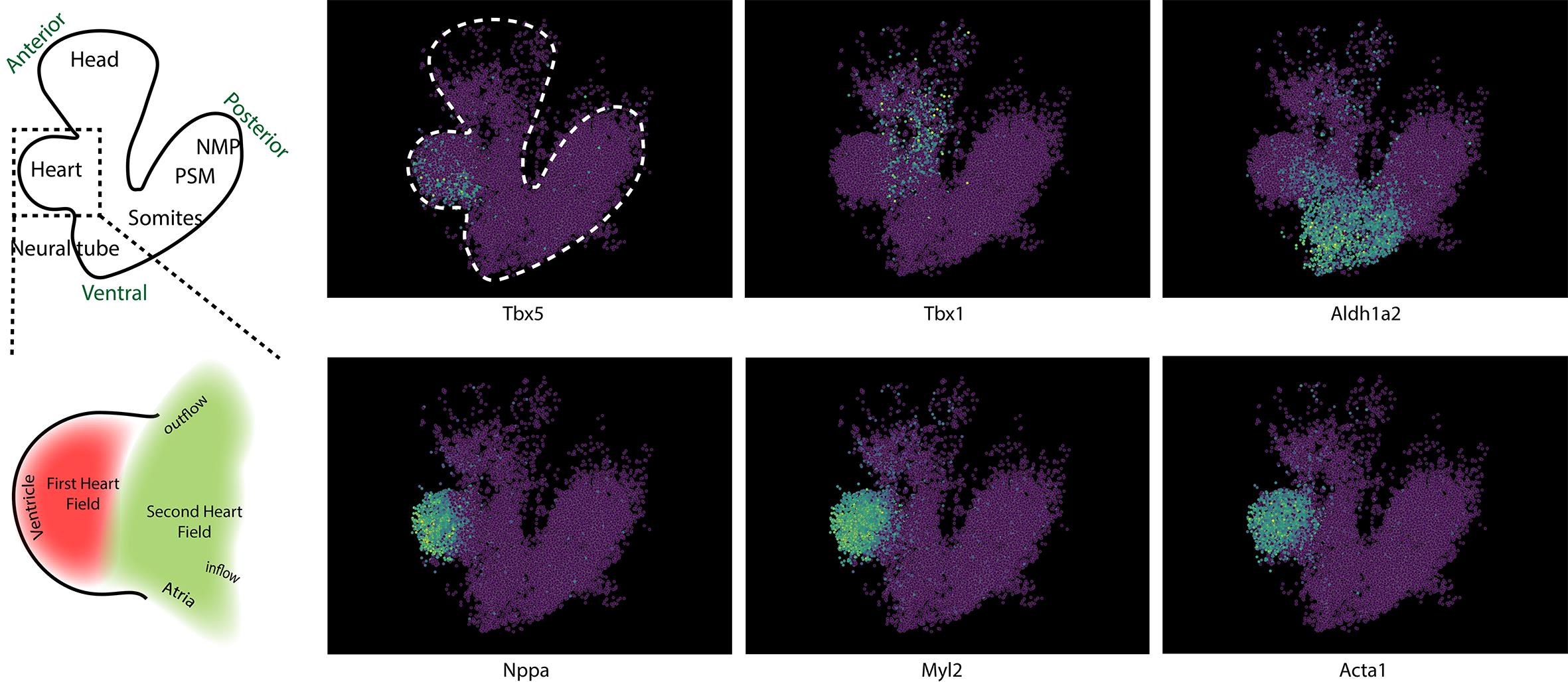
Figure 9. Validation of cardiac patterning in the reconstructed E8.5 heart. Representative spatial expression patterns of key cardiac genes in the reconstructed E8.5 heart tube. On the left, a diagram (top) and its heart inset (down) are shown for clarification. On the top images, Tbx5 marks the first heart field (FHF), which contributes mainly to the left ventricle and parts of the atria; Tbx1 labels progenitors of the second heart field (SHF) located in the pharyngeal mesoderm that give rise to the outflow tract and right ventricle; and Aldh1a2 (Raldh2) identifies the posterior/inflow pole, where retinoic acid signaling patterns atrial myocardium. On the bottom images, within the differentiated myocardium, Nppa (ANF), Myl2 (MLC-2v), and Acta1 are enriched in the contractile ventricular cardiomyocytes. The reconstructed expression domains reproduce the known spatial organization of the early mouse heart: FHF-derived ventricle (Tbx5+/Myl2+), SHF-derived outflow tract (Tbx1+), and atrial inflow ( Aldh1a2+/Nppa+), confirming that the 3D alignment preserves biological geometry.
To assess its usability across datasets and sequencing techniques, we applied sc3D to the publicly available MOSTA E16.5 mouse embryo dataset, consisting of Stereo-seq spatial transcriptomic sections [19]. For this dataset, individual .h5ad section files were harmonized and merged using Code S2, which standardizes column names and metadata formats (e.g., obs["orig.ident"], obsm["X_spatial"], and obs["predicted.id"]) before input into the main reconstruction pipeline (Code S1). After registration, sc3D successfully aligned the serial sections into coherent 3D coordinate systems, preserving the anatomical continuity of major organ systems, including the neural tube, somites, heart, lung, liver, and developing kidney (Video 1). The resulting reconstructions captured tissue contours and consistent spatial alignment across slices, showing that the registration performs well in independently generated spatial datasets.

To evaluate whether sc3D preserves developmental transcriptional gradients, we used sc3D napari viewer to analyze Hox cluster gene expression along the anterior–posterior axis, a hallmark of vertebrate spatial patterning [20,21]. The virtual in situ hybridizations (vISH) of Hoxa2–Hoxa10 revealed spatially ordered, progressively posterior domains of expression that reflected their genomic organization along the HoxA cluster (Video 1). Early anterior members, such as Hoxa2 and Hoxa3, were restricted to the hindbrain and cervical regions, while posterior genes ( Hoxa7–Hoxa10) extended caudally along the trunk and tail bud. These gradients reproduced canonical Hox collinearity and positional identity rules described during vertebrate embryogenesis, validating the spatial reconstruction [20,21]. The continuity of these patterns across sections demonstrates that sc3D can bridge local 2D expression domains into global 3D morphogenetic coordinates. Together, these results show that sc3D generalizes across spatial transcriptomic datasets from different species and sequencing technologies, maintaining spatial fidelity and enabling quantitative analysis of molecular gradients.
Limitations and potential failure modes: Like other slice-based spatial reconstruction approaches, sc3D assumes consistent section thickness and sufficient spatial sampling across consecutive slices. Large variability in slice thickness, missing sections, or strong nonlinear tissue distortions (for example, due to folding, tearing, or uneven mounting) can reduce registration accuracy and may lead to local misalignment. Similarly, datasets with low bead or spot density, sparse gene detection, or limited tissue coverage may provide insufficient spatial information for reliable correspondence estimation. In practice, visual inspection of reconstructed volumes, evaluation of tissue continuity across sections, and sensitivity analyses using alternative parameter settings are recommended to identify potential failure cases and to ensure robust interpretation of the results. This has been tested for the E8.5 datasets; the analysis and instructions can be found in Figure 3f of [14].
General notes and troubleshooting
Reproducibility
All analyses were performed using sc3D (v3.0.0) and the companion Jupyter notebooks provided as Supplementary Material (Code S1, S2). The workflow was executed on a macOS system (version 15.6.1, ARM64 architecture, chip M1, 10-core CPU, 32 GB RAM) using the following environment (Table 3):
Table 3. Software environment and version information
| Component | Version/specification |
| Python | 3.13 (packaged by conda-forge) |
| NumPy | 2.4.1 |
| Platform | macOS-15.6.1-arm64 |
| Compiler | Clang 18.1.8 |
| Processor | Apple M-series ARM64 |
| sc3D | 3.0.0 |
| AnnData | 0.12.7 |
| Scanpy | 1.10.2 |
| Matplotlib | 3.10.8 |
| Napari/napari-sc3D-viewer | 0.5.4/2.0.0 |
The workflow was run in an isolated mamba environment to ensure dependency control and reproducibility. All notebooks were executed successfully under this configuration without requiring GPU acceleration. We recommend Python 3.13.
General notes
1. Column overrides: If your AnnData uses different names, pass tissue_id, array_id, pos_id, gene_name_id, pos_reg_id to SpatialOmicArray(...).
2. Genes of interest: Provide markers spanning major germ layers to assess registration quality visually.
3. Memory management: For full atlases (>500k beads), use Stage C downsampling before showing in napari.
Troubleshooting
Problem 1: Registration artifacts (twists or discontinuities).
Probable causes: Incorrect slice ordering or large inter-slice gaps, or the presence of small or poorly segmented tissue clusters that bias alignment.
Solutions: Verify 'orig.ident' numeric order; increase `nb_CS_begin_ignore`/`nb_CS_end_ignore` to drop edge slices; consider excluding unstable clusters via tissues_to_ignore and adjusting th_d if pairings are too sparse or too permissive.
Problem 2: Missing registered coordinates.
Probable causes: Early termination or wrong column names.
Solutions: Check .obsm content; re-run Stage A and ensure pos_id=X_spatial if your position column differs.
Example error messages:
KeyError: 'X_spatial'KeyError: 'X_spatial_registered'AttributeError: 'SpatialOmicArray' object has no attribute 'pos_3D'Problem 3: Napari freezes on load.
Probable causes: Excessive bead count or large gene matrix.
Solutions: Use the minimal/downsampled file; hide low-variance genes.
Example error messages:
MemoryError: Unable to allocate arraynumpy.core._exceptions._ArrayMemoryErrorProblem 4: Memory errors during interpolation or visualization.
Probable causes: Large bead counts, dense gene matrices, or excessive interpolation.
Solutions: Downsample the dataset before interpolation, reduce nb_interp, or increase available RAM. Avoid plotting many genes simultaneously; focus on selected tissues or genes.
Supplementary information
The following supporting information can be downloaded here:
1. Code S1. Jupyter notebook to reproduce step-by-step this protocol.
2. Code S2. Jupyter notebook to load the E16.5 MOSTA (or your own data) slices, merge them into a single AnnData object, verify spatial metadata consistency, and save the merged object to run it in the sc3D notebook (Code S1).
Acknowledgments
Conceptualization, L.G. and A.B.; Methodology, M.S.; Software and workflow adaptation, M.S. and L.G.; Writing, M.S.; Review and Editing, A.B. and L.G.; Supervision, L.G.
We thank all authors of the original publication [14] for their contributions to the development and validation of the sc3D method, and members of the Meissner and Guignard laboratories for valuable discussions during its implementation. We are also grateful to the developers of anndata, scanpy, and napari for providing open-source infrastructure that made this protocol possible. The figshare team is acknowledged for hosting the raw and registered datasets used here. This work was supported by institutional funding from CENTURI: French National Research Agency (“France 2030”, ANR-16-CONV-0001 from Excellence Initiative of Aix-Marseille University - A*MIDEX).
Competing interests
The authors declare no competing interests.
References
- Bolondi, A., Law, B. K., Kretzmer, H., Gassaloglu, S. I., Buschow, R., Riemenschneider, C., Yang, D., Walther, M., Veenvliet, J. V., Meissner, A., et al. (2024). Reconstructing axial progenitor field dynamics in mouse stem cell-derived embryoids. Dev Cell. 59(12): 1489–1505.e14. https://doi.org/10.1016/j.devcel.2024.03.024
- Fruleux, A., Hong, L., Roeder, A. H. K., Li, C. B. and Boudaoud, A. (2024). Growth couples temporal and spatial fluctuations of tissue properties during morphogenesis. Proc Natl Acad Sci USA. 121(23): e2318481121. https://doi.org/10.1073/pnas.2318481121
- McDaniel, C., Simsek, M. F., Chandel, A. S. and Özbudak, E. M. (2024). Spatiotemporal control of pattern formation during somitogenesis. Sci Adv. 10(4): eadk8937. https://doi.org/10.1126/sciadv.adk8937
- Asp, M., Giacomello, S., Larsson, L., Wu, C., Fürth, D., Qian, X., Wärdell, E., Custodio, J., Reimegård, J., Salmén, F., et al. (2019). A Spatiotemporal Organ-Wide Gene Expression and Cell Atlas of the Developing Human Heart. Cell. 179(7): 1647–1660.e19. https://doi.org/10.1016/j.cell.2019.11.025
- Ji, A. L., Rubin, A. J., Thrane, K., Jiang, S., Reynolds, D. L., Meyers, R. M., Guo, M. G., George, B. M., Mollbrink, A., Bergenstråhle, J., et al. (2020). Multimodal Analysis of Composition and Spatial Architecture in Human Squamous Cell Carcinoma. Cell. 182(2): 497–514.e22. https://doi.org/10.1016/j.cell.2020.05.039
- Maynard, K. R., Collado-Torres, L., Weber, L. M., Uytingco, C., Barry, B. K., Williams, S. R., Catallini, J. L., Tran, M. N., Besich, Z., Tippani, M., et al. (2021). Transcriptome-scale spatial gene expression in the human dorsolateral prefrontal cortex. Nat Neurosci. 24(3): 425–436. https://doi.org/10.1038/s41593-020-00787-0
- Long, Y., Ang, K. S., Sethi, R., Liao, S., Heng, Y., van Olst, L., Ye, S., Zhong, C., Xu, H., Zhang, D., et al. (2024). Deciphering spatial domains from spatial multi-omics with SpatialGlue. Nat Methods. 21(9): 1658–1667. https://doi.org/10.1038/s41592-024-02316-4
- Sun, S., Liu, J., Li, G. and Liu, B. (2025). DeepGFT: identifying spatial domains in spatial transcriptomics of complex and 3D tissue using deep learning and graph Fourier transform. Genome Biol. 26(1): 153. https://doi.org/10.1186/s13059-025-03631-5
- Yu, Y. and Xie, Z. (2024). Spatial Transcriptomic Alignment, Integration, and de novo 3D Reconstruction by STAIR. Res Squ. https://doi.org/10.21203/rs.3.rs-3939678/v1
- Wolf, F. A., Angerer, P. and Theis, F. J. (2018). SCANPY: large-scale single-cell gene expression data analysis. Genome Biol. 19(1): 15. https://doi.org/10.1186/s13059-017-1382-0
- Sendra, M., de Dios Hourcade, J., Temiño, S., Sarabia, A. J., Ocaña, O. H., Domínguez, J. N. and Torres, M. (2023). Cre recombinase microinjection for single-cell tracing and localised gene targeting. Development. 150(3): e201206. https://doi.org/10.1242/dev.201206
- Oliveira, M. F. d., Romero, J. P., Chung, M., Williams, S. R., Gottscho, A. D., Gupta, A., Pilipauskas, S. E., Mohabbat, S., Raman, N., Sukovich, D. J., et al. (2025). High-definition spatial transcriptomic profiling of immune cell populations in colorectal cancer. Nat Genet. 57(6): 1512–1523. https://doi.org/10.1038/s41588-025-02193-3
- Pavlopoulos, A. and Wolff, C. (2020). Crustacean Limb Morphogenesis during Normal Development and Regeneration. In Anger, K., Harzsch, S. and Thiel, M. (Eds.). Developmental Biology and Larval Ecology (1st ed.). Oxford University Press. 46–79. https://doi.org/10.1093/oso/9780190648954.003.0002
- Sampath Kumar, A., Tian, L., Bolondi, A., Hernández, A. A., Stickels, R., Kretzmer, H., Murray, E., Wittler, L., Walther, M., Barakat, G., et al. (2023). Spatiotemporal transcriptomic maps of whole mouse embryos at the onset of organogenesis. Nat Genet. 55(7): 1176–1185. https://doi.org/10.1038/s41588-023-01435-6
- Zeira, R., Land, M., Strzalkowski, A. and Raphael, B. J. (2022). Alignment and integration of spatial transcriptomics data. Nat Methods. 19(5): 567–575. https://doi.org/10.1038/s41592-022-01459-6
- Bruneau, B. G., Nemer, G., Schmitt, J. P., Charron, F., Robitaille, L., Caron, S., Conner, D. A., Gessler, M., Nemer, M., Seidman, C. E., et al. (2001). A Murine Model of Holt-Oram Syndrome Defines Roles of the T-Box Transcription Factor Tbx5 in Cardiogenesis and Disease. Cell. 106(6): 709–721. https://doi.org/10.1016/s0092-8674(01)00493-7
- Sendra, M., Domínguez, J., Torres, M. and Ocaña, O. (2021). Dissecting the Complexity of Early Heart Progenitor Cells. J Cardiovasc Dev Dis. 9(1): 5. https://doi.org/10.3390/jcdd9010005
- Kelly, R. G., Buckingham, M. E. and Moorman, A. F. (2014). Heart Fields and Cardiac Morphogenesis. Cold Spring Harb Perspect Med. 4(10): a015750–a015750. https://doi.org/10.1101/cshperspect.a015750
- Chen, A., Liao, S., Cheng, M., Ma, K., Wu, L., Lai, Y., Qiu, X., Yang, J., Xu, J., Hao, S., et al. (2022). Spatiotemporal transcriptomic atlas of mouse organogenesis using DNA nanoball-patterned arrays. Cell. 185(10): 1777–1792.e21. https://doi.org/10.1016/j.cell.2022.04.003
- Duboule, D. and Dollé, P. (1989). The structural and functional organization of the murine HOX gene family resembles that of Drosophila homeotic genes. EMBO J. 8(5): 1497–1505. https://doi.org/10.1002/j.1460-2075.1989.tb03534.x
- Mallo, M. and Alonso, C. R. (2013). The regulation of Hox gene expression during animal development. Development. 140(19): 3951–3963. https://doi.org/10.1242/dev.068346
Article Information
Publication history
Received: Dec 10, 2025
Accepted: Jan 18, 2026
Available online: Feb 6, 2026
Published: Feb 20, 2026
Copyright
© 2026 The Author(s); This is an open access article under the CC BY-NC license (https://creativecommons.org/licenses/by-nc/4.0/).
How to cite
Sendra, M., Bolondi, A. and Guignard, L. (2026). sc3D: A Comprehensive Tool for 3D Spatial Transcriptomic Analysis. Bio-protocol 16(4): e5607. DOI: 10.21769/BioProtoc.5607.
Category
Bioinformatics and Computational Biology
Systems Biology > Spatial transcriptomics
Molecular Biology > DNA > Gene expression
Do you have any questions about this protocol?
Post your question to gather feedback from the community. We will also invite the authors of this article to respond.