- Protocols

- Articles and Issues
- For Authors
- About
- Become a Reviewer

Whole-Mount Immunostaining for the Visual Separation of A- and C-Fibers in the Study of the Sciatic Nerve
Published: Vol 15, Iss 23, Dec 5, 2025 DOI: 10.21769/BioProtoc.5529 Views: 1460
Reviewed by: Olga KopachAnonymous reviewer(s)
Original research article
The authors used this protocol in:

Dec 2024

Protocol Collections
Comprehensive collections of detailed, peer-reviewed protocols focusing on specific topics


Related protocols
Abstract
Peripheral nerve injuries (PNIs) often result in incomplete functional recovery due to insufficient or misdirected axonal regeneration. Balanced regeneration of myelinated A-fibers and unmyelinated C-fibers is essential for functional recovery, making it crucial to understand their differential regeneration patterns to improve PNI treatment outcomes. However, immunochemical staining does not clearly differentiate between A- and C-fiber axons in whole-mount nerve preparations. To overcome this limitation, we developed a modified protocol by optimizing the immunostaining to restrict the antibody access to myelinated axons. This enables visualization of A-fibers by myelin sheath labeling, while allowing selective staining of unmyelinated C-fiber axons. As a result, A- and C-fibers can be reliably distinguished, facilitating accurate analysis of their regeneration in both normal and post-injury conditions. Combined with confocal microscopy, this approach supports efficient screening of whole-mount nerve preparations to evaluate fiber density, spatial distribution, axonal sprouting, and morphological characteristics. The refined technique provides a robust tool for advancing PNI research and may contribute to the development of more effective therapeutic strategies for nerve repair.
Key features
• Visual separation of myelinated A-fibers and unmyelinated C-fibers is achieved by restricting the penetration of axon-labeling antibodies through the myelin sheaths.
• The protocol also distinguishes A- and C-fibers based on the types of associated Schwann cells.
• The protocol is specially designed to distinguish between A- and C-fibers as well as their morphological features in whole-mount nerve preparations.
• The protocol does not require specialized reagents, equipment, or techniques, making it highly accessible and reproducible across different research settings.
Keywords: Peripheral nerveGraphical overview

Background
Peripheral nerve injury (PNI) is a common and challenging clinical problem that often results in irreversible motor and sensory deficits, affecting patients’ quality of life and placing a burden on healthcare systems [1]. PNI can arise from various causes, including domestic and combat injuries, surgical procedures, or certain medical conditions. Unlike the central nervous system (CNS), the peripheral nervous system (PNS) has a much higher capacity for regeneration [2–4]. Nevertheless, despite this innate regenerative potential, functional recovery following PNS injuries is often incomplete and slow, especially in the case of severe or extensive nerve damage [5]. Morphological assessment of peripheral nerve recovery after PNI commonly relies on histological techniques, including the preparation of tissue sections, their subsequent immunohistostaining, and visualization. However, those techniques present significant challenges, especially when preparing transverse or longitudinal sections of nerves with small diameters and considerable lengths. Such preparation increases the risk of tissue damage, which may compromise the accuracy of subsequent morphometric analysis and raise concerns about the reliability of extrapolating the findings to the entire nerve. Furthermore, these procedures are typically labor-intensive and require costly equipment and reagents that may not always be readily available.
To address these limitations, the whole-mount staining (WMS) technique has gained increasing popularity in recent years. Unlike traditional sectioning methods, WMS allows three-dimensional visualization of axonal regeneration, providing a more comprehensive depiction of nerve tissue architecture and the spatial patterns of axonal sprouting [6,7]. This significantly enhances our understanding of the mechanisms underlying neural regeneration, especially when combined with advanced imaging techniques such as confocal microscopy [8].
The growing popularity of these techniques highlights the need to better understand the different regeneration patterns of myelinated A-fibers and unmyelinated C-fibers after PNI within the WMS preparation. Aα-fibers are among the most heavily myelinated fibers, responsible for transmitting efferent signals to muscles and involved in motor function of the peripheral nerve, conducting signals at speeds of 30–120 m/s. Another highly myelinated type is the afferent muscle spindles, or Aβ fibers, which carry tactile and proprioceptive signals from skin and joints at similar speeds [9]. Aδ-fibers are myelinated, medium-diameter axons involved in sensory function, particularly in the perception of sharp pain and temperature, with conduction velocities of 5–30 m/s [10,11]. The axons of rat myelinated fibers in the sciatic nerve are 1–5 μm in diameter, with mean values of ~2.5 μm, depending on the animal age and location within the nerve. In contrast, C-fibers, which mediate diffuse pain and thermal sensitivity at slower conduction velocities (0.5–2 m/s), have unmyelinated axons with diameters of 0.1–3.0 μm, substantially overlapping those of A-fibers [10]. Besides, small-diameter unmyelinated axons are not evenly distributed and often form bundles of many axons [10], having diameters comparable to those of A-fibers. So, standard WMS techniques emerged to overcome the 2D limitation by preserving the structural integrity of the tissue. However, these methods still fail to clearly distinguish between myelinated A-fibers and unmyelinated C-fibers, largely due to the similar diameters of small A-fibers and C-fiber bundles, as well as signal overlap from axonal markers.
Our methodology overcomes these issues by enhancing signal specificity and minimizing marker colocalization, thereby enabling clear and reliable differentiation between A- and C-fibers in WMS preparations of peripheral nerves. This approach facilitates a more effective, precise tracking of their respective regeneration patterns and offers a valuable tool for advancing PNI research. It is well known that A-fibers are myelinated, while C-fibers are unmyelinated [10,11]. This morphological arrangement might influence the accessibility of antibodies to protein markers. Myelin basic protein (MBP), located in the myelin sheaths, is accessible for immunostaining even after mild permeabilization. In contrast, the neurofilament heavy chain (NfH) protein is located within axons, which, in the case of A-fibers, are ensheathed by myelin, potentially limiting NfH antibody penetration. We hypothesized that modifying the concentrations of Triton X-100 (TX100) and bovine serum albumin (BSA) in the blocking solution would prevent NfH antibody access to A-fiber axons and selectively visualize C- rather than A-fibers. Nonetheless, A-fibers could be visualized by MBP antibody staining. To test this, we optimized the concentrations of these components to achieve selective labeling, thereby facilitating further morphological differentiation of these fiber types.
Materials and reagents
Biological materials
1. Male Wistar rats (2–5 months old, 200–450 g)
Reagents
1. Diethyl ether (Synthesia, catalog number: 60-29-7)
2. Sodium chloride (NaCl) (Sigma, catalog number: S-9625)
3. Heparin, 180 USP units/mg (Merck, catalog number: H3393-10KU)
4. Paraformaldehyde (PFA) (Sigma-Aldrich, catalog number: P6148)
5. Sodium hydroxide (NaOH) (MilliporeSigma, catalog number: S8045)
6. Sodium phosphate monobasic monohydrate (H2NaO4P·H2O) (Sigma-Aldrich, catalog number: 71504)
7. Sodium phosphate dibasic (HNa2O4P) (Sigma-Aldrich, catalog number: 04276)
8. Bovine serum albumin (BSA) (Sigma, catalog number: A-7906)
9. Triton X-100 (Sigma, catalog number: T9284)
10. Primary antibodies (Table 1)
11. Secondary antibodies (Table 2)
Table 1. List of tested primary antibodies
| Target | Source | Dilution | Manufacturer |
|---|---|---|---|
| Myelin basic protein (MBP) | Rabbit | 1:1,000 | Abcam, catalog number: ab40390, RRID:AB_1141521 |
| Myelin basic protein (MBP) | Rabbit | 1:500 | Novus Biological, catalog number: NB100-7983 |
| S100 | Mouse | 1:1,000 | Abcam, catalog number: ab34686, RRID:AB_777793 |
| Neurofilament heavy chain (NfH) | Chicken | 1:5,000 | Abcam, catalog number: ab4680, RRID:AB_304560 |
Table 2. List of tested secondary antibodies
| Target | Source | Fluorophore | Dilution | Manufacturer |
|---|---|---|---|---|
| Rabbit IgG | Donkey | Alexa Fluor 488 | 1:500 | Invitrogen, catalog number: A-21206, RRID:AB_2535792 |
| Rabbit IgG | Goat | Alexa Fluor 647 | 1:500 | Invitrogen, catalog number: A-27040, RRID:AB_2536101 |
| Mouse IgG | Goat | Alexa Fluor 488 | 1:500 | Invitrogen, catalog number: A-21121, RRID:AB_2535764 |
| Mouse IgG | Donkey | Alexa Fluor 555 | 1:500 | Invitrogen, catalog number: A-31570, RRID:AB_2536180 |
| Mouse IgG | Donkey | Alexa Fluor 647 | 1:500 | Jackson ImmunoResearch Labs, catalog number: 715-605-151, RRID:AB_2340863 |
| Chicken IgY | Goat | Alexa Fluor 488 | 1:500 | Invitrogen, catalog number: A-11039, RRID:AB_2534096 |
| Chicken IgY | Goat | Alexa Fluor 647 | 1:500 | Abcam, catalog number: ab150171, RRID:AB_2921318 |
Solutions
1. 0.9% NaCl (see Recipes)
2. 12% PFA (see Recipes)
3. 0.2 M phosphate buffer (PB) (see Recipes)
4. 10% Triton X-100 (see Recipes)
5. 10% bovine serum albumin (see Recipes)
6. Blocking solution (see Recipes)
7. Antibody dilution solution (see Recipes)
Recipes
1. 0.9% NaCl (w/v)
| Reagent | Final concentration | Quantity or volume |
|---|---|---|
| NaCl | 0.9% (w/v) | 4.5 g |
| ddH2O | n/a | 500 mL |
| Total | n/a | 500 mL |
Note: Prepare the solution immediately before transcardial perfusion to ensure it remains fresh. If needed, store at 4 °C for up to 1 month.
2. 12% PFA (w/v), pH 7.4
| Reagent | Final concentration | Quantity or volume |
|---|---|---|
| PFA | 12% (w/v) | 60 g |
| NaOH, 2 M | n/a | 2 mL |
| ddH2O | n/a | 498 mL |
| Total | n/a | 500 mL |
Notes:
1. For transcardial perfusion and fixation of tissues, 4% PFA must be used within 48 h after preparation. Therefore, it is better to prepare a 3× stock solution (12% PFA), which can be diluted just before use.
2. 2 M NaOH is used to adjust the pH of solution to 7.4. The volume indicated is approximate.
a. Make all procedures in a fume hood.
b. Dissolve 60 g of PFA in 500 mL of ddH2O using a magnetic stirrer with a hotplate at 40–50 °C.
Note: The boiling point is 60 °C; be careful not to overheat or boil your solution. To prevent the vaporization of the solution, it is better to cover the glass beaker with foil!
c. For better dissolution, add 2 mL of 2 M NaOH. The solution with fully dissolved PFA is opalescent and nearly transparent.
d. Filter the mixture using a vacuum pump.
e. Store the solution in glassware at 4 °C for up to 3 months.
f. Right before use, dilute the solution three times; the final concentration should be 4%.
3. 0.2 M phosphate buffer (PB), pH 7.4
| Reagent | Final concentration | Quantity or volume |
|---|---|---|
| HNa2O4P | 0.1 M | 6.9 g |
| ddH2O (for dissolving HNa2O4P) | n/a | 250 mL |
| H2NaO4P·H2O | 0.1 M | 22.72 g |
| ddH2O (for dissolving H2NaO4P·H2O) | n/a | 800 mL |
| Total | n/a | 1,050 mL |
a. Take 6.9 g of HNa2O4P and dissolve it in 250 mL of ddH2O using a magnetic stirrer at room temperature (RT) to prepare dibasic sodium phosphate.
b. To prepare monobasic sodium phosphate, put 22.72 g of H2NaO4P·H2O inside another glass beaker and dissolve it in 800 mL of ddH2O using a magnetic stirrer at RT.
c. Adjust the pH of dibasic sodium phosphate to 7.4 with monobasic sodium phosphate by checking it with a pH meter.
d. Store solution at 4 °C for up to 3 months. The formation of crystals at the bottom of your solution after preparation and storage at 4 °C for at least 2 days is normal and indicates that the solution was made correctly.
e. Before usage, heat 0.2 M PB at 37 °C and dilute it to 0.1 M PB with ddH2O.
4. 10% Triton X-100 (v/v)
| Reagent | Final concentration | Quantity or volume |
|---|---|---|
| Triton X-100 | 10% | 10 mL |
| ddH2O | n/a | 90 mL |
| Total | n/a | 100 mL |
Note: Triton X-100 is extremely viscous and difficult to pipette accurately. Preparing the solution may be time-consuming.
a. Add 10 mL of Triton X-100 to 80 mL of ddH2O in a glass beaker.
b. Use a magnetic stirrer on a low speed setting at RT. Avoid vortexing or high-speed stirring as this will create excessive foam.
c. Once fully dissolved, transfer the solution to a 100 mL graduated cylinder and add ddH2O to bring the final volume to 100 mL.
d. Store solution at 4 °C for up to 3 months or at -20 °C up to 6 months.
5. 10% Bovine serum albumin (w/v)
| Reagent | Final concentration | Quantity or volume |
|---|---|---|
| BSA | 10% | 10 g |
| PB, 0.1 M (see Recipe 3) | n/a | 90 mL |
| Total | n/a | 100 mL |
a. Add 80 mL of 0.1 M PB to a glass beaker with a magnetic stir bar. Use a magnetic stirrer on a low speed setting at RT.
b. Slowly add 10 g of BSA onto the surface of the stirring PB.
Note: Do not put all the BSA at once, as it will form large clumps that are very difficult to dissolve.
c. Once fully dissolved, transfer dissolved solution to a 100 mL graduated cylinder and add ddH2O to bring the final volume to 100 mL.
d. Store solution at 4 °C for up to 1 month or at -20 °C up to 6 months.
6. Blocking solution
| Reagent | Final concentration | Quantity or volume |
|---|---|---|
| Triton X-100, 10% (v/v; see Recipe 4) | 1% | 50 μL |
| BSA, 10% (w/v; see Recipe 5) | 9% | 450 μL |
| Total | n/a | 500 μL |
Notes:
1. All calculations are made per one well of a 24-cell well plate.
2. The volume of the blocking solution should be at least two times the volume of solutions with diluted primary and secondary antibodies for proper blocking, not only to prevent unspecific binding sites on samples but also to block cells on the plate to prevent antibody binding with them.
3. Prepare immediately before usage.
7. Antibody dilution solution
| Reagent | Final concentration | Quantity or volume |
|---|---|---|
| Triton X-100, 10% (v/v; see Recipe 4) | 0.3% | 7.5 μL |
| BSA, 10% (w/v; see Recipe 5) | 5% | 125 μL |
| PB, 0.1 M (see Recipe 3) | n/a | 117.5 μL |
| Total | n/a | 250 μL |
Notes:
1. All calculations are made per one well of a 24-cell well plate.
2. Prepare immediately before usage.
Laboratory supplies
1. 6-well cell culture plates (Falcon, catalog number: 353046)
2. 24-well cell culture plates (Cellstar, catalog number: 662160 or Falcon, catalog number: 353047)
3. Microcentrifuge tubes, 0.6 mL (Fisher Scientific, catalog number: 02-681-311)
4. Microcentrifuge tubes, 1.5 mL (Deltalab, catalog number: 200400P)
5. Pipette tips, 0.1–10 μL (VWR, catalog number: 89041-382)
6. Pipette tips, 2–200 μL (Deltalab, catalog number: 200016A)
7. Pipette tips, 100–1,000 μL (Deltalab, catalog number: 200012)
8. Cell culture dishes, 35 × 10 mm (Cellstar, catalog number: 627160)
9. Filter paper (e.g., Munktell Filtrak, catalog number: 110069)
10. Slice hold-down (Warner Instruments, catalog number: 64-0255)
11. Parafilm M (Parafilm, catalog number: PM-996)
12. Graduated cylinder, 250 mL (any available)
13. Glass beakers, 250 mL, 500 mL, and 1 L (any available)
14. Dissection pad (you can use a foam pad wrapped in aluminum foil)
15. Desiccator (any one available that fits an animal)
16. Cotton wool (any available)
17. Nitrile gloves (any available)
18. Needles (any available)
Equipment
A. Laboratory equipment
1. Pipette, 0.1–2.5 μL (Eppendorf, catalog number: 3123000012)
2. Pipette, 0.5–10 μL (Eppendorf, catalog number: 3123000020)
3. Pipette, 10–100 μL (Eppendorf, catalog number: 3123000047)
4. Pipette, 100–1,000 μL (Eppendorf, catalog number: 3123000063)
5. Scales (any available)
6 Analytical balance (Ohaus, model: VP214C)
7. Magnetic stirrer with hotplate (Joanlab, model: HS5Pro)
8. pH meter (Mettler Toledo, model: FiveEasy Plus)
9. Vacuum pump (Joanlab, model: VP-10L)
10. Laboratory water bath (any available)
11. Fume hood (any available)
12. Peristaltic pump (e.g., Thermo Fisher Scientific, catalog number: 13-876-4)
13. 3D oscillating laboratory shaker (Joanlab, model: OS-30Pro)
B. Tools for transcardial perfusion and isolation of the sciatic nerve
1. Curved iris scissors, 11.5 cm (e.g., World Precision Instruments, catalog number: 501759)
2. Straight operating scissors, 14 cm (e.g., World Precision Instruments, catalog number: 14192)
3. Curved Rochester-Ochsner hemostatic forceps, 16.0 cm (e.g., World Precision Instruments, catalog number: 501710)
4. Scalpel handle (e.g., World Precision Instruments, catalog number: 500237)
5. Scalpel blade, #24 (e.g., World Precision Instruments, catalog number: 500247)
6. Tweezer forceps, 12 cm (e.g., World Precision Instruments, catalog number: 500338)
7. Curved micro scissors, 12 cm (e.g., World Precision Instruments, catalog number: 503364)
C. Imaging
1. Stereomicroscope (Olympus, model: SZX7)
2. Laser scanning confocal microscope (Olympus, model: FV1000)
3. Objective, 10 × 0.3 (Olympus, model: UPLFLN10X2)
4. Objective, 20 × 0.5 (Olympus, model: UPLFLN20X)
5. Water-dipping objective, 40 × 0.8 (Olympus, model: LUMPLFLN40XW)
6. Water-dipping objective, 60 × 1.0 (Olympus, model: LUMPLFLN60XW)
Software and datasets
1. For imaging: FV10-ASW (Olympus, version: 4.1); requires a license
2. For image processing: ImageJ (version: 1.54g, available at https://imagej.net/)
3. For image analysis:
a. Python (version: 3.12, available at https://www.python.org/)
b. Miniconda (available at https://docs.anaconda.com/)
c. napari [12] (available at https://napari.org/)
4. For data analysis:
a. R (version: 4.4.2, available at https://www.cran.r-project.org/)
b. RStudio (version: 2024.09.1, available at https://posit.co/products/open-source/rstudio/)
c. RTools (version: 4.4, available at https://www.cran.r-project.org/)
d. nervecount-napari (version: 0.1.0-beta [13], available at https://github.com/valusty/nervecount-napari)
Note: Software for image analysis and data analysis was used in this article solely for validation purposes on confocal images of transverse sections, not whole-mount preparations.
Procedure
A. Transcardial perfusion
Figure 1 shows a suggested scheme, illustrating key points during transcardial perfusion.

Figure 1. Key steps during transcardial perfusion. (A) A vertical incision is made in the skin to expose the thoracic cavity. Arrows indicate the direction of the incision. (B) Opening the chest to expose the heart. (Ba) Lateral incisions are made under the ribcage to expose the diaphragm (marked in cyan). (Bb) The diaphragm is carefully cut to access the heart. Arrows show the direction of the incision. (C) Preparing the heart for perfusion. (Ca) The right atrium (marked in green) is incised to allow blood to flow out. The heart is outlined in white. (Cb) A needle (marked in red) connected to the perfusion system is inserted into the left ventricle (marked in magenta) for the inflow of perfusion solutions. Other parts of the heart are outlined in white. (Cc) Close-up image showing the allocation of the needle (marked in red) during perfusion. (D) Performing perfusion. (Da) Perfusion begins with a 0.9% NaCl solution containing heparin to prevent clotting and flush out blood. (Db) Successful perfusion is indicated by the lightening of the heart (white) and liver (yellow) due to blood washout.
Caution: All steps must be performed in a flow hood.
1. Wipe all working surfaces and tools with ethanol.
2. Prepare a solution of 0.9% NaCl (see Recipe 1).
Note: For perfusion, 1 mL of 0.9% NaCl is required per 2 g of animal weight.
3. Dilute a solution of 12% PFA (see Recipe 2) to a concentration of 4%.
Note: For perfusion, 1 mL of 4% PFA is required per 2 g of animal weight. For better tissue fixation, ice-cold PFA is recommended.
4. Heat 0.9% NaCl to 37 °C and add heparin to a final concentration of 80 IU/kg of animal weight.
Notes:
1. We use a heparinized 0.9% NaCl solution (saline) during the initial perfusion stage to efficiently flush blood from the circulatory system. This is a standard and effective method to prevent clotting and ensure that the subsequent fixative (4% PFA) perfuses tissues thoroughly and achieves optimal preservation.
2. If you perfuse more than one animal, perform this step separately for each animal immediately before perfusion.
5. Prepare the peristaltic pump for perfusion. Rinse all components and tubes with ddH2O and 0.9% NaCl solution. Ensure all tubing is free of air bubbles.
Note: If you perfuse more than one animal, perform this step right before perfusion for each animal separately.
6. To perform inhalation anesthesia, put an animal in a desiccator containing cotton wool and a small amount of diethyl ether.
Critical: The use of diethyl ether is actually a historical method. Modern, safer anesthetics such as isoflurane administered via a vaporizer, injectable ketamine/xylazine, etc., are recommended. Adhere to your institution’s approved animal care and use approved protocols.
Caution: To prevent the spread of diethyl ether odor, ensure the lid of the desiccator is tightly fitted. It is necessary to keep a constant eye on it, as an awake animal may open the lid. Store diethyl ether in a well-ventilated area only!
Note: During anesthesia with diethyl ether, the animal's breathing should be monitored. For 450 g rats, the maximum time is 7 min, and the average is 2–3 min. Some animals may experience difficulty falling asleep, which can lead to respiratory arrest.
7. Carefully put and secure the anesthetized rat on the dissection pad by ensuring the four legs are secured with needles.
Critical: The animal must be in a deep surgical plane of anesthesia before beginning the perfusion, confirmed by a negative pedal reflex (tested by the toe pinch test). For a procedure of this duration, if available, a continuous administration system (e.g., isoflurane vaporizer) or an appropriate long-acting injectable anesthetic is recommended to maintain a stable depth of anesthesia throughout.
8. Gain access to the heart of the rat:
a. Pull back the animal’s skin on the sternum and make a vertical incision and subsequent cuts laterally using straight operating scissors to expose the thoracic cavity (Figure 1A).
b. When the xiphoid bone is visible, gently make lateral incisions under the chest to open the diaphragm and liver.
c. Carefully cut the diaphragm and make two incisions on both sides of the chest up to the clavicle. Using hemostat forceps, lift the xiphoid bone, thus opening access to the heart and lungs (Figure 1B).
9. Cut the right atrium (Figure 1C).
Note: The correct section will be indicated by an instantaneous flow of venous blood, which has a dark red color.
10. Carefully insert the needle connected to the perfusion system tube into the left ventricle of the heart at an angle approximately parallel to the midline of the heart.
Caution: Do not insert the needle too deeply to avoid disrupting the midline of the heart.
11. After all surgical procedures, start perfusion with 0.9% NaCl solution containing heparin; the NaCl supply rate is 10 mL/min, to wash out blood from the large circulation circle (Figure 1C).
Note: A sufficient level of blood washout is indicated by a noticeable lightening of the liver color and by transparency of the circulating blood (Figure 1D).
12. Stop the perfusion system to prevent air from entering the tubing.
13. Replace the perfusion solution with a 4% PFA and restart the perfusion system.
Note: The proper tissue fixation is indicated by muscle contraction, tail twitching, and nose hardening.
14. After perfusion, remove the needle from the left ventricle.
15. Remove the animal from the dissection pad.
B. Isolation of the sciatic nerve
Figure 2 shows a suggested scheme, illustrating key points during the isolation of the sciatic nerve.

Figure 2. Key steps involved in isolating the sciatic nerve. (A) Dorsal side of a perfused rat with the skin exposed. A straight incision (indicated by the white dashed arrow) was made along the projection of the femur (outlined in green). (B) The overlying muscles were carefully dissected to expose the sciatic nerve (outlined in yellow). The direction of further dissection of the sciatic nerve from surrounding connective tissue and muscles using curved iris scissors is indicated by white arrows. The direction of an additional skin incision necessary for proper access to the sciatic nerve is shown with a black arrow. (C) The sciatic nerve and its branches are isolated from the surrounding tissue. The approximate sites for further nerve dissection are marked with yellow dashed lines.
1. Turn the body of the perfused rat to expose the dorsal side.
2. Use straight operating scissors to cut the skin along the projection of the femur.
Note: If you need to isolate two sciatic nerves, remove the skin over the entire thigh by gradually cutting the connective tissue between the skin and muscle. For simplicity, the skin should be pulled as it is removed.
3. Use a scalpel to dissect the muscles along the line of the sciatic nerve (Figure 2A). Make cuts in the muscle tissue carefully and smoothly to avoid damage to the nerve.
4. Gently separate the sciatic nerve from the connective tissue and muscles using curved iris scissors (Figure 2B).
5. Dissect a section of the sciatic nerve localized from its exit point from the spinal canal to the point where it divides into three branches (Figure 2C). Use curved iris scissors and avoid applying tension to the nerve, which can cause deformation.
Note: If needed, for these branches, you should perform steps B4–5 for each branch. If you do not need branches for further research, it is still better to isolate the nerve with them for holding without any disruption of the sciatic nerve.
6. Transfer the isolated sciatic nerves to a small piece of filter paper and spread them out with forceps.
7. Place the filter paper with the sciatic nerve into the 6-well cell plate for a post-fixation with 4% PFA for 24 h at 4 °C.
Critical: Monitor the post-fixation time to avoid excessive tissue fixation, which may interfere with normal immunohistostaining.
C. Epineurium removal
Figure 3 shows a suggested scheme, illustrating key points during epineural removal.
1. Place the isolated sciatic nerve in a cell culture dish containing 0.1 M PB.
2. Position the dish with the sciatic nerve under a stereomicroscope against a dark background for better visualization.
3. Perform further operations under 2× optical magnification to see the epineurium during removal.
4. Gently fix the nerve without firm compression at the proximal end using tweezers forceps (Figure 3A).
5. Start by slightly undercutting the epineurium at the proximal end and spreading it apart.
6. Use a pair of tweezers to carefully pull the epineurium toward the distal end while holding the nerve in place with another pair of tweezers (Figure 3B).
7. Continue this process until the epineurium is entirely removed.
8. Put the fixed nerve with the removed epineurium in 0.1 M PB and store it at 4 °C.

Figure 3. Key steps during epineurium removal. (A) The sciatic nerve is placed in a cell culture dish containing 0.1 M phosphate buffer (PB). The nerve is gently stabilized at the proximal end (PS, outlined in white) and distally (DS, outlined in black) using tweezers forceps. A slight incision is made at the PS of the nerve to undercut the epineurium. (B) One pair of tweezers (highlighted in black) is used to carefully pull the epineurium toward the DS, while another pair (highlighted in white) holds the nerve in place. Arrows indicate the direction of epineurium removal. (C) The nerve after the epineurium removal.
D. Immunohistochemistry
1. Incubate the samples in blocking solution (see Recipe 4) at 4 °C with constant shaking using a 3D oscillator shaker at 80 rpm with a tilt angle of 10° in a 24-well plate for 24 h.
2. Right before immunostaining, dilute chosen primary antibodies (see Table 1) in antibody dilution solution (see Recipe 5) in the following combinations:
a. MBP (rabbit) + NfH (chicken).
b. MBP (rabbit) + S100 (mouse).
3. Incubate the samples with primary antibodies in antibody dilution solution for 72 h at 4 °C with constant shaking at 80 rpm with a tilt angle of 10°.
4. Wash samples with 0.1 M PB three times for 15 min at RT with constant shaking at 80 rpm with a tilt angle of 10°.
5. Right before immunostaining, dilute the chosen secondary antibodies (see Table 2) in antibody dilution solution.
6. Incubate the samples with secondary antibodies in antibody dilution solution for 2 h at RT with constant shaking at 80 rpm with a tilt angle of 10° in the following combinations:
a. For the combination in step D2a: Alexa 488 anti-rabbit + Alexa 647 anti-chicken or Alexa 647 anti-rabbit + Alexa 488 anti-chicken.
b. For the combination in step D2b: Alexa 488 anti-rabbit + Alexa 647 anti-mouse or Alexa 647 anti-rabbit + Alexa 488 anti-mouse.
7. Wash the samples three times for 15 min in 0.1 M PB.
8. Store stained nerves in 0.1 M PB at 4 °C, protected from light. Stained samples can be stored for at least two weeks without significant signal loss.
E. Confocal microscopy
1. Transfer the sample to a cell culture dish with 0.1 M PB.
2. Use a slice hold-down to fix the sample in one position.
3. Place the sample on the stage of a laser scanning confocal microscope. Ensure the microscope stage is stable to prevent sample movement during imaging.
4. Image whole-mount stained nerve to study the general pattern of regeneration of nervous tissue and its vascularization using a 10× objective with an NA of 0.3 at a pinhole size of 785–800 μm. Alternatively, use a 20× objective with an NA of 0.5 and a pinhole size of 400–500 μm for higher magnification.
5. For a more detailed and local study of axon regeneration, perform confocal imaging using a 40 water-dipping objective with an NA of 0.8 at a pinhole size of 200–400 μm. Alternatively, use a 60× objective with an NA of 1.0 at a pinhole size of 200–400 μm for higher magnification.
6. Choose optimal settings for samples using the HiLo pseudocolor image look-up table (LUT) to cover the whole dynamic range in your setting.
7. Optimize laser intensity and exposure time to minimize photobleaching and ensure consistent fluorescence intensity across images.
Note: The pinhole sizes mentioned are optimal for our setting. However, it is essential to adjust the pinhole size as needed to optimize resolution and signal-to-noise ratio for each objective used.
8. For further analysis, maximum intensity projection (MIP) images were used to create a 2D representation from the 3D Z-stack, providing a comprehensive view of the nerve fiber architecture within the imaged volume.
F. Data analysis
Note: Images were acquired from a minimum of three distinct regions per nerve sample, with at least three animals per experimental group.
1. Qualitative analysis of whole-mount preparations:
a. The A-to-C-fiber ratio was assessed qualitatively in whole-mount preparations and supported by quantitative density analysis from sections.
b. Axonal sprouting was identified morphologically by the presence of fine, branching nerve fibers deviating from the main axon tracts.
2. Quantitative morphometric analysis of nerve transverse sections:
a. For the morphometric analysis of nerve transverse sections, the nervecount-napari plugin was used, which is designed for the segmentation of immunofluorescent images [13]. The entire processing pipeline was automated using the Analyze function, which sequentially performs preprocessing (background correction, maximum intensity projection, and median filtering), segmentation (Multi-Otsu thresholding and morphological opening), and object separation (watershed segmentation).
b. Following segmentation, the Quantify all function was used to measure and export morphometric parameters for each individual axon, including area, axis lengths, and intensity. This data, along with summary statistics (e.g., total number of labels, axon area as a percentage of the total image area), was saved as .csv files for further analysis.
c. Statistical analysis was performed using a Kruskal–Wallis test followed by Dunn’s multiple comparison test.
Validation of protocol
A. Differentiating between A- and C-fibers using MBP and NfH staining
After experimenting with a composition of blocking solutions, we decided to use one containing 9% BSA and 1% TX100. Under these conditions, MBP and NfH were stained with their respective antibodies and visualized using confocal microscopy in the terminal region of the stained sciatic nerve of naïve animals enriched by A-fibers. The myelin sheaths of A-fibers were clearly visible in this sciatic nerve preparation (Figure 4Aa). At the same time, A-fiber axons were not stained by the NfH antibody and were not observed inside the myelin sheaths (Figure 4Ab,c). Next, we validated that the NfH antibodies can potentially stain axons of A-fibers. We suggested that there were many terminal ends of the fibers in this part of the nerve with exposed axonal sections, which the NfH antibodies can stain. Indeed, we observed dotted NfH staining at the terminals of A-fibers visualized by MBP staining, while no fluorescence corresponding to the signal of axons was detected inside the myelin sheaths, marked by MBP (Figure 4Aa–4Ae).

Figure 4. Max-projection confocal images of a whole-mount immunostained sciatic nerve under optimized permeabilization conditions for selective visualization of A- and C-fibers. Z-stack depth ~20 μm. (A, B) Representative regions from different nerve variants. (A) Terminal region of a nerve containing both A- and C-fibers, with a predominance of A-fibers. Clusters of terminal ends of A-fibers are marked by arrowheads. (Aa) Myelin basic protein staining (MBP, green) of myelinated A-fibers. (Ab) Neurofilament heavy chain staining (NfH, red) of unmyelinated C-fibers. NfH staining is absent in A-fibers, except in exposed axon sections at fiber terminals. (Ac) Overlay of (Aa) and (Ab). (Ad) Magnified view of the region of interest (ROI) (marked by magenta dashed lines in Aa, Ab, and Ac), showing A-fibers with NfH signal at exposed fiber ends, which is consistent with axonal staining at cut sites. (Ae) Magnified view of the ROI (marked by green dashed lines in Aa, Ab, and Ac), showing visible C-fibers (marked by arrows), running parallel to A-fibers. (B) Higher magnification image of another nerve tissue variant illustrating both A-fibers and C-fibers (marked by arrows). (Ba) MBP staining of myelinated A-fibers. (Bb) C-fibers are observed by NfH staining. (Bc) Overlay of (Ba) and (Bc). (Bd) Magnified view of the ROI (marked by yellow dashed lines in Ba, Bb, and Bc) showing predominantly A-fibers and thin C-fibers (marked by arrows) with a diameter less than 2 μm. (Be) Magnified view of the ROI (marked by cyan dashed lines in Ba, Bb, and Bc), highlighting the nodes of Ranvier (marked by an asterisk).
In general, NfH fluorescence within A-fibers was predominantly observed in areas where fibers were sectioned or damaged (Figure 4A). The absence of NfH fluorescence inside myelin sheaths indicates the impossibility of NfH antibody penetration through the sheaths in chosen experimental conditions, while NfH staining of A-fiber terminals demonstrates that A-fiber axons can be potentially stained. This result is crucial for separating myelinated and unmyelinated fibers.
In most regions of the WMS preparations, visible axons can be detected by antibodies against NfH (Figure 4Bb). These axons were observed outside of the myelin sheaths running in parallel to A-fibers (Figure 4Ba,c). A part of these axons had diameters of up to 2 μm, which corresponds to diameters of non-myelinated C-fibers. Frequently, these axons were observed in close opposition to each other, suggesting that bundles of Remak were detected (Figure 4Bb,d). In some cases, red dots of NfH staining with two attached short strips were observed inside the A-fibers (Figure 4Be). We suggest that nodes of Ranvier were better exposed to the NfH antibodies, resulting in staining of A-fiber axons in their vicinity, observed as the dots (axonal segment in the node of Ranvier) with short strips of neighboring axons. Usually, just a few such dots with strips were observed per field of view (0.317 × 0.317 mm), despite the presence of numerous A-fibers. This observation aligns with the idea that myelinating Schwann cells ensheath single large-diameter axons and form compact myelin over internodal segments typically spanning ~1 mm in adult rats [14].
Thus, this series of experiments confirms that A- and C-fibers can be reliably distinguished using MBP and NfH immunostaining, respectively. Moreover, damaged A-fibers and their nodes of Ranvier, as well as the bundles of Remak, can be visualized in the WMS preparation using this approach. These features provide a robust framework for assessing changes in fiber composition and the functional state of A-fibers during development, PNI, and therapeutic interventions targeting PNI.
B. Differentiation A- and C-fibers using MBP and S100 staining
Since our goal in this research was to identify different populations of peripheral nerve fibers, we also aimed to distinguish between myelinated A-fibers and unmyelinated C-fibers based on their association with specific types of glial cells, namely, myelinating and non-myelinating Schwann cells (SCs). The myelin basic protein, a marker solely expressed in the myelin sheaths, localizes around A-fibers and serves as a reliable indicator of myelinating Schwann cells (mSCs). In contrast, S100, a protein commonly localized in the cytoplasm and nuclei as well as in Schmidt-Lanterman incisures and paranodal loops at the node of Ranvier of Schwann cells [15], labels both mSCs and non-myelinating Schwann cells, also known as Remak Schwann cells (RSCs). RSCs form Remak bundles, which mainly consist of unmyelinated C-fiber axons, each separated by the membranous processes of the RSC rather than being directly in contact with its cytoplasm. An increased density of Remak bundles has been associated with increased sensitivity to thermal and mechanical stimuli, and, in some cases, impaired motor coordination [16,17], establishing them as a relevant morphological marker. While MBP is specific for myelinating SCs and A-fibers, S100 labels both SC subtypes, making it useful for visualizing the overall SC distribution. Additionally, C-fibers may potentially be visualized through association with S100, but not with MBP labeling. Studying the ratio of mSCs and RSCs can serve as a helpful indicator to evaluate the ratio of A- and C-fibers, which, in turn, can assist in estimating the effectiveness of new treatment approaches for PNI [16].
To assess the feasibility of the proposed approach, we performed immunolabeling of S100 and MBP in sciatic nerve preparations of naïve animals. As expected, no complete signal colocalization was observed, reflecting the distinct subcellular localizations of these proteins. MBP was distributed relatively randomly across the thickness of A-fibers (Figure 5Aa), whereas S100 was predominantly localized to their outermost layer, corresponding to the cytoplasmic domain of Schwann cells (Figure 5Ab).
In regions where S100 and MBP staining overlapped, A-fibers typically appeared as broad, straight green strips (MBP stained) flanked by two narrow red strips (S100 stained) (Figure 5Ac, Bc). Schwann cell nuclei and adjacent cytoplasm were exclusively labeled by S100, with no detectable MBP signal (Figure 5Ac, Bc). These findings are consistent with previous observations demonstrating that myelinating Schwann cells are elongated and straight along the axon. In contrast, RSCs envelop multiple small-diameter unmyelinated axons within Remak bundles, extending over ~100–300 μm longitudinally. Their cytoplasm follows the tortuous paths of C-fibers, resulting in a wavy, undulating morphology [18,20]. In some regions, S100 staining appeared as a single wavy broad red strip with minimal or absent MBP labeling (Figure 5Ab, Bb), which likely corresponds to SCs associated with unmyelinated C-fibers, forming the Remak bundles.
Notably, MBP labeling of A-fibers revealed a banded pattern, with an MBP signal markedly reduced or absent in irregular transverse bands spaced tens of microns apart (Figure 5Ba). In contrast, S100 staining was elevated or did not change in the same regions (Figure 5Bb), suggesting the presence of Schwann cell cytoplasm. These bands most likely represent Schmidt-Lanterman incisures—cytoplasmic clefts that interrupt the otherwise compact myelin sheath. There are 5–20 such structures in each myelinating Schwann cell that facilitate metabolic exchange, organelle transport, and the maintenance of myelin [19]. Their number per internode and structural organization are important for nerve regeneration [19] and maintenance [21,22] as well as for action potential propagation [21]. The identification of Schmidt-Lanterman incisures provides an additional advantage for analyzing structural changes in A-fibers during sciatic nerve regeneration.
Thus, we have demonstrated that co-labeling distinct Schwann cell markers in WMS sciatic nerve preparations enables the assessment of the numbers of A- vs. C-fibers as well as certain morphological features of A-fibers, such as the nodes of Ranvier and Schmidt-Lanterman incisures.

Figure 5. Max-projection confocal images of nerve fibers illustrating myelinating and non-myelinating Schwann cells (SCs). Z-stack depth ~20 μm. (A) Representative field of view and (B) magnified view of a region of interest (ROI) marked in (A) by cyan. (Aa) Myelin basic protein (MBP, green) for visualization of myelin sheaths, specifically marking myelinating SCs (mSCs) associated with A-fibers. Somata of SCs marked by the arrowhead. Schmidt-Lanterman incisures are marked by arrows. SCs associated with non-myelinating C-fibers are marked by asterisks. (Ab) Immunolabeling for glial cell cytoplasmic protein S100 protein (red) identifies both myelinating SCs (mSCs) and non-myelinating Remak SCs (RSCs). (Ac) Overlay of (Aa) and (Ab). (B) Magnified view of the ROI (marked by cyan dashed lines in Aa, Ab, and Ac). Somata of SCs marked by the arrowhead. Schmidt-Lanterman incisures are marked by arrows. SCs associated with non-myelinating C-fibers are marked by an asterisk. (Ba) MBP (green) for visualization of myelin sheaths, specifically marking mSCs associated with A-fibers. (Bb) S100 (red) labels both mSCs and RSCs. (Bc) Overlay of (Ba) and (Bb).
To confirm that the absence of NfH staining in A-fiber axons is not due to interference from MBP staining of myelinating Schwann cells, we performed additional immunolabeling using an antibody against S100 protein, a distinct SC marker. S100 is predominantly localized to the outermost cytoplasmic layer of SCs [16] and does not colocalize with MBP. It is localized at a distance from A-fiber axons, making it unlikely to interfere with NfH staining.
A sciatic nerve preparation of naïve rats was co-labeled for S100 and NfH using the developed protocol (9% BSA and 1% TX100). The resulting staining patterns closely resembled those observed with MBP/NfH co-labeling. S100 reliably marked SCs associated with A-fibers (Figure 6Aa), while NfH appeared as red puncta in regions corresponding to cross-sections of myelinated A-fibers (Figure 6Ab). Notably, the spatial distribution of S100 and MBP within SCs was clearly distinct: S100 was confined to the narrow outer cytoplasmic layer, whereas MBP was concentrated in the inner layers surrounding the axons (compare Figure 5Aa and Figure 6Aa). As with MBP/NfH co-labeling, dotted NfH staining was most prominent in the terminal region of the sciatic nerve, where damaged A-fibers are enriched (Figure 6Ac). Additionally, thin fibers (<2 μm in diameter) labeled by NfH antibodies were frequently observed (Fig. 6Bb). These likely represent unmyelinated C-fiber axons, similar to those seen in MBP/NfH preparations (Figure 4Bb). Unlike MBP, S100 labeling partially surrounded these C-fibers, reflecting cytoplasmic staining of SCs (Figure 6Bc). This partial overlap of S100 and NfH signals supports the presence of RSCs, which are not detected by MBP staining due to the absence of MBP expression in these cells. In some preparations, we also observed bundles of thin fibers enveloped by diffuse S100 staining (Figure 6C), consistent with bundles of Remak.

Figure 6. Max-projection confocal images of whole-mount sciatic nerve preparations immunolabeled to visualize Schwann cell (SC) distribution and associated axons, enabling distinction between myelinated A-fibers and unmyelinated C-fibers. Z-stack depth ~20 μm. (A–C) Representative regions from different nerve variants to illustrate distinct morphological features. (A) Regions showing strong neurofilament heavy chain (NfH) fluorescence predominantly in cuts of myelinated A-fiber areas, consistent with the localization of myelin basic protein (MBP) in myelinating SCs (mSCs). Cross-sections of myelinated A-fibers and bundles of Remak are marked by arrowheads. (Aa) Glial cytoplasmic protein S100 (green), expressed in both mSCs and non-myelinating Remak SCs (RSCs). (Ab) NfH-labeled axons (red). NfH signal is absent within the myelin sheaths except at the cut edges of nerve fibers. (Ac) Overlay of (Aa) and (Ab). (B) Areas of another nerve variant containing thin, clearly visible axons partially surrounded by S100-labeled SCs cytoplasm, likely corresponding to low-myelinated Aδ fibers or unmyelinated C-fibers. Cross-sections of myelinated A-fibers marked by arrowheads. C-fibers marked by arrows. (Ba) S100 (green) staining. (Bb) NfH (red) staining. (Bc) Overlay of (Ba) and (Bb). (C) Regions of another nerve variant demonstrating partial overlap of S100 and NfH signals, indicating non-myelinating RSCs enclosing multiple C-fibers in Remak bundles. Cross-sections of myelinated A-fibers are marked by arrowheads. Bundles of Remak are marked by arrows. (Ca) S100 (green) labeling of RSCs cytoplasm. (Cb) NfH (red) labeling of C-fiber axons. (Cc) Overlay of (Ca) and (Cb) showing cytoplasmic encapsulation of multiple axons within Remak bundles.
Nevertheless, regardless of the used set of antibodies, our labeling protocol reliably distinguished A- and C-fibers. This differentiation is likely achieved through selective NfH labeling of C-fibers and the lack of NfH signal in A-fiber axons, which are surrounded by SCs and instead labeled by MBP.
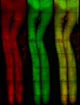
To further validate that the NfH antibody failed to label A-fiber axons due to restricted access caused by surrounding myelinating Schwann cells, we modified the protocol to enhance Schwann cell permeability. We hypothesized that increasing sheath permeability would allow the NfH antibody to penetrate the myelin and access A-fiber axons. Indeed, by adjusting the blocking solution to contain 7% BSA and 3% TX100, we achieved effective permeabilization of the myelin sheaths, enabling NfH antibody penetration (Figure 7). Under these conditions, both A- and C-fiber axons were successfully stained (Figure 7B). However, such staining compromised the ability to distinguish between fiber types, as the enhanced permeability resulted in uniform labeling across the axonal population. While this modification allows for comprehensive visualization of axons in WMS sciatic nerve preparations, we opted to retain the original protocol that limits antibody access through the myelin sheath. This ensures clear visual separation between myelinated and unmyelinated axons, which is critical for subtype-specific analysis.

Figure 7. Max-projection confocal images of a whole-mount stained nerve treated with a blocking solution containing 7% BSA and 3% Triton X-100, demonstrating enhanced antibody penetration through myelin sheaths. Z-stack depth ~20 μm. (A) Glial cell cytoplasmic protein S100 (green) for visualization of Schwann cells. (B) Neurofilament heavy chain (NfH, red) for visualization of axons. (C) Overlay of (A) and (B).
At the distal end of the examined preparations, the rat sciatic nerve contains approximately 27,000 axons, of which 6% are myelinated motor fibers, 23% are myelinated sensory fibers, 48% are unmyelinated sensory fibers, and 23% are unmyelinated sympathetic fibers [23]. Notably, the unmyelinated sympathetic axons are absent at the proximal end of the nerve, resulting in a relative composition of 37% myelinated and 63% unmyelinated fibers in that region.
Our immunofluorescence data reveal a pronounced shift in the A-to-C-fiber ratio, favoring A-fibers (Figures 4–6). This observation is consistent with the imaging constraints inherent to our whole-mount preparations and fiber distribution in sciatic nerve fascicles. Specifically, confocal imaging was limited to the outer surface of the fascicles following epineurium removal, and Z-stack depths for maximum projection images rarely exceeded ~20 μm. Moreover, antibody penetration into the deeper regions of the fascicles was likely suboptimal, which contributed to a reduced fluorescence signal in the tissue core. It is well-established that myelinated A-fibers are preferentially located at the periphery of nerve fascicles, whereas unmyelinated C-fibers are concentrated centrally [24]. Therefore, the observed bias toward A-fibers likely reflects the superficial sampling of the fascicle’s architecture inherent to our imaging approach.
To summarize, our findings demonstrate that the protocol we employed is effective and reliable for examining nerve structure. This approach can be utilized in future studies to assess the effectiveness of treatments aimed at enhancing nerve regeneration following peripheral nerve injuries.
C. Application of the optimized protocol to a model of peripheral nerve injury
Finally, we applied the developed protocol for differentiating A- and C-fibers to assess changes in fiber composition in a rat model of PNI involving silicone conduit implantation. A 10 mm-long silicone tube (inner diameter: 1 mm; outer diameter: 2 mm) was implanted to bridge a 6 mm gap of the sciatic nerve. This model allows for the assessment of nerve regeneration across a defined defect. After five months, the animals were sacrificed, and segments of the ipsilateral sciatic nerve, including the conduit and adjacent proximal and distal regions, along with the corresponding contralateral sciatic nerve, were excised. The silicone tube was carefully removed, and both the regenerated tissue and the contralateral nerve were stained for MBP and NfH using the optimized protocol.
Staining of the contralateral sciatic nerve revealed features consistent with those observed in control animals (compare Figure 4B and Figure 8A). Within the conduit, regenerating fibers predominantly extended along the longitudinal axis of the nerve, closely resembling the alignment seen in the contralateral, uninjured nerve (Figure 8Bb,d). However, a marked shift in the A-to-C-fiber ratio was evident. The majority of axons within the regenerated tissue were unmyelinated C-fibers (Figure 8Bb,d), whereas the contralateral nerve primarily consisted of myelinated A-fibers (Figure 8A), as revealed by the same staining protocol. The bundles of Remak were also not observed in the PNI model. Overall, the presence of mSCs within the conduit was minimal, indicating significantly impaired remyelination (Figure 8B). The possible sites of axonal sprouting were also observed (Figure 8Be).

Figure 8. Max-projection of confocal images of whole-mount stained sciatic nerves under normal conditions and after injury. Z-stack depth ~20 μm. (A) Representative region from control (contralateral) sciatic nerve showing normal axonal organization and myelination, with clear visualization of both A-fibers and C-fibers. (Aa) Myelin basic protein (MBP, green) showing myelin sheaths of A-fibers. (b) Neurofilament heavy chain (NfH, red) showing C-fiber axons. Within A-fibers, the NfH signal is absent, except at fiber terminals or cut edges. (c) Overlay of (Aa) and (Ab). (B) Representative region from the regenerated tissue within an injured sciatic nerve (ipsilateral nerve of the same animal) with an implanted silicone conduit 20 weeks after surgery. Regenerating axons within the tube are primarily aligned parallel to the rostrocaudal axis, resembling the organization of axons in the contralateral nerve. However, myelinating Schwann cells are nearly absent within the tube, indicating impaired remyelination. (Ba) MBP (green) for visualization of myelin sheaths. (Bb) NfH (red) for visualization of axons. (Bc) Overlay of (Ba) and (Bb). (Bd) Magnified view of the region of interest (ROI) (marked by magenta dashed lines in Ba, Bb, and Bc) showing the normal, parallelly aligned distribution of axons within the conduit. (Be) Magnified view of the ROI (marked by green dashed lines in Ba, Bb, and Bc), highlighting spots of axonal sprouting within the regenerated tissue (marked by arrows). Axonal sprouting was identified by the presence of fine, branching nerve fibers deviating from the main axon tracts.
Notably, the total number of axons, encompassing both A- and C-fibers, was higher in the regenerated tissue compared to the contralateral nerve, supporting possible axonal sprouting during regeneration. In particular, quantitative analysis of axon numbers per field of view (317 × 317 μm ) in transverse sections showed that axon density within the silicone tube (median [range]: 1467 [480; 2072]; n = 3 animals/3 nerves/7 sections) was significantly higher than in both proximal (736 [583; 989]; n = 3/3/13) and distal segments (726 [317; 1511]; n = 3/3/53) of the contralateral nerve (p ≤ 0.001).
Our findings demonstrate that the optimized blocking solution effectively prevents anti-NfH antibodies from penetrating the myelin of A-fibers, while still allowing reasonable antibody access to the axons of C-fibers, thereby supporting both specific NfH staining of C-fibers and strong MBP staining of the myelin sheaths of A-fibers. This selective labeling allows reliable distinction between A- and C-fibers in WMS preparations. In addition, we showed that co-labeling distinct SC markers in WMS sciatic nerve preparations also enables assessment of A- vs. C-fibers and analyses of certain morphological features of A-fibers. These methods may serve as useful tools for structural analysis of peripheral nerves both under normal conditions and after peripheral injuries.
General notes and troubleshooting
General notes
1. We developed a protocol by modifying the blocking solution composition. Specifically, we adjusted the concentrations of BSA for blocking and TX100 for permeabilization. Our optimized protocol utilizes a blocking solution with 9% BSA and 1% TX100. This adjustment allowed for the visualization of myelin sheaths labeled with anti-MBP antibodies, while preventing the penetration of anti-NfH antibodies through the myelin sheaths.
2. Intra-sheath NfH fluorescence was absent inside MBP+ regions, coupled with sporadic colocalization in small-diameter fibers (≤2 μm), corresponding to unmyelinated C-fibers. These findings suggest that a higher BSA concentration, combined with low TX100 presence, leads to lower penetration levels of anti-NfH antibodies through myelin sheaths. Additionally, it shows that a lower concentration of TX100 has not affected the myelin sheaths, thus ensuring the preservation of the samples’ structural integrity. To validate this hypothesis, we tested other combinations of component concentrations, including 7% BSA and 3% TX100. This adjustment increased antibody penetration, resulting in detectable intra-sheath NfH fluorescence within myelinated fibers. These results demonstrate that the proportions of blocking solution affect antibody accessibility and signal separation during confocal imaging.
3. Compared with previous protocols, our method integrates an optimized blocking solution that precisely controls antibody penetration, enabling the clear visual separation of myelinated A-fibers and unmyelinated C-fibers. Unlike conventional approaches that rely on labor-intensive 2D sectioning or standard whole-mount methods suffering from signal overlap, our technique ensures reproducibility, accessibility, and preserves the native 3D architecture of the nerve. Figures 4–6 illustrate the superior structural clarity and differential staining achieved.
4. This protocol is primarily designed for studying peripheral nerve regeneration in the sciatic nerve of Wistar rats. However, it can be adapted with appropriate adjustments in other model organisms or for answering different scientific questions. For example, it can be adapted for studying nerve regeneration in different species (such as mice), other nerves, or under various pathological conditions (including other types of PNI, inflammatory responses, chronic pain, and their impact on A- and C-fibers distribution and proportions).
5. Variability in staining results can arise from factors such as the quality of antibodies, the freshness of reagents, and the handling of samples before and during the staining process. To minimize variability, ensure that all reagents are appropriately stored and used within their shelf life.
6. This protocol is optimized for WMS and may not be compatible with tissue-clearing techniques. Caution is advised when attempting to integrate this protocol with optical clearing methods.
7. The protocol is primarily designed for qualitative assessment of nerve fibers and SC using WMS. However, due to limitations in imaging resolution and antibody penetration, it may not be suitable for accurate quantitative analysis of parameters such as fiber diameter or density. To address these limitations, the protocol is used as a preparatory step before creating transverse sections for further quantitative analysis. After WMS, tissues are sectioned to enable a detailed examination of nerve fiber morphology and SC distribution. Given the limited penetration of antibodies through thicker tissue samples, an additional round of staining is performed on the transverse sections. This approach ensures qualitative visualization of fibers and allows precise quantitative analysis while minimizing the number of animals required for the study.
8. For robust quantitative analysis, it is recommended to acquire images from a minimum of three distinct regions per nerve sample (e.g., proximal stump, distal stump, and, in the case of the PNI model, the spot of injury and subsequent regeneration), with at least three animals per experimental group.
9. Mounting whole-mount nerves on a standard glass slide with a coverslip is not recommended, as it can compress the tissue. Alternatives for stabilizing the tissue without compression include using specialized imaging chambers or creating a small well on a slide with spacers.
Troubleshooting
Problem 1: Poor antibody penetration and weak staining.
Possible causes: Insufficient permeabilization, inadequate blocking solution, or poor quality of antibodies.
Solutions: Slightly increase the concentration of Triton X-100 in the blocking solution, ensure proper storage and handling of antibodies, and verify the expiration dates of reagents.
Problem 2: High background staining.
Possible causes: Overly concentrated antibodies, insufficient washing.
Solutions: Dilute the antibodies with a higher dilution rate and increase the number of washes.
Problem 3: Inconsistent staining across samples.
Possible causes: Variability in tissue handling, fixation quality, or differences in reagent batches.
Solutions: Standardize tissue preparation and fixation protocols, use reagents from the same batch for all samples, and ensure consistent incubation times and temperatures to achieve reproducible results.
Problem 4: Difficulty in visualizing specific markers.
Possible causes: Improper marker specificity, insufficient antibody concentration, or poor imaging settings.
Solutions: Use alternative antibodies with higher specificity, adjust the concentration of antibodies, and optimize imaging settings (e.g., gain, exposure time, pinhole) to enhance signal detection.
Acknowledgments
Methodology, V.U.; Investigation, V.U., T.P.; Conceptualization, V.U., P.B., V.M.; Writing – Original Draft, V.U.; Writing – Review & Editing, P.B., T.P., N.V., V.M.; Funding acquisition, N.V.; Supervision, T.P., P.B.
This research was funded by NRFU grant # 2021.01/0328 to N.V. and the National Academy of Science of Ukraine grants (0124U001556 and 0124U001557). V.U. is supported by the NASU PhD school.
During the preparation of this work, the authors used the AI-assisted tool Grammarly to improve the language of the manuscript and its readability. After using this tool, the authors reviewed and edited the content as needed and take full responsibility for the content of the published article.
Image panels were created using the open-source vector graphics image editor Inkscape. The Graphical overview was created using Adobe Illustrator for iPad and Inkscape.
Competing interests
The authors have declared no competing interests.
Ethical considerations
Two-month-old male Wistar rats (240–280 g) were used in this study. Rats were housed in cages under standard, controlled conditions with a 12/12 h day/night cycle at 20–23 °C. Laboratory food and water were available ad libitum.
Bioethical regulations were approved by the Committee on Biomedical Ethics of the Bogomolets Institute of Physiology (Protocol No. 2.24 of 22.05.2024). All research protocols comply with the provisions of the Council of Europe Convention on Bioethics (1997), the European Convention for the Protection of Vertebrate Animals Used for Experimental and Other Scientific Purposes (Strasbourg, 1986), the General Ethical Principles of Scientific Research adopted by the First National Congress of Ukraine on Bioethics (September 2001), and the Law of Ukraine No. 3447-IV “On Protection of Animals from Cruelty” (2006).
References
- Lopes, B., Sousa, P., Alvites, R., Branquinho, M., Sousa, A. C., Mendonça, C., Atayde, L. M., Luís, A. L., Varejão, A. S. P., Maurício, A. C., et al. (2022). Peripheral Nerve Injury Treatments and Advances: One Health Perspective. Int J Mol Sci. 23(2): 918. https://doi.org/10.3390/ijms23020918
- Lavorato, A., Aruta, G., De Marco, R., Zeppa, P., Titolo, P., Colonna, M. R., Galeano, M., Costa, A. L., Vincitorio, F., Garbossa, D., et al. (2023). Traumatic peripheral nerve injuries: a classification proposal. J Orthop Traumatol. 24(1): e1186/s10195–023–00695–6. https://doi.org/10.1186/s10195-023-00695-6
- Tomé, D. and Almeida, R. D. (2024). The injured axon: intrinsic mechanisms driving axonal regeneration. Trends Neurosci. 47(11): 875–891. https://doi.org/10.1016/j.tins.2024.09.009
- Nagappan, P. G., Chen, H. and Wang, D. Y. (2020). Neuroregeneration and plasticity: a review of the physiological mechanisms for achieving functional recovery postinjury. Mil Med Res. 7(1): 1–16. https://doi.org/10.1186/s40779-020-00259-3
- Juckett, L., Saffari, T. M., Ormseth, B., Senger, J. L. and Moore, A. M. (2022). The Effect of Electrical Stimulation on Nerve Regeneration Following Peripheral Nerve Injury. Biomolecules. 12(12): 1856. https://doi.org/10.3390/biom12121856
- Dun, X. p. and Parkinson, D. B. (2015). Visualizing Peripheral Nerve Regeneration by Whole Mount Staining. PLoS One. 10(3): e0119168. https://doi.org/10.1371/journal.pone.0119168
- Dun, X. P. and Parkinson, D. B. (2018). Whole Mount Immunostaining on Mouse Sciatic Nerves to Visualize Events of Peripheral Nerve Regeneration. Methods Mol Biol. 1739: 339–348. https://doi.org/10.1007/978-1-4939-7649-2_22
- Jung, Y., Ng, J. H., Keating, C. P., Senthil-Kumar, P., Zhao, J., Randolph, M. A., Winograd, J. M. and Evans, C. L. (2014). Comprehensive Evaluation of Peripheral Nerve Regeneration in the Acute Healing Phase Using Tissue Clearing and Optical Microscopy in a Rodent Model. PLoS One. 9(4): e94054. https://doi.org/10.1371/journal.pone.0094054
- Menorca, R. M. G., Fussell, T. S. and Elfar, J. C. (2013). Peripheral Nerve Trauma: Mechanisms of Injury and Recovery. Hand Clin. 29(3): 317. https://doi.org/10.1016/J.HCL.2013.04.002
- Kanda, T. (2000). Pathological changes of human unmyelinated nerve fibers: a review. Histol Histopathol, 15(1), 313–324. https://doi.org/10.14670/HH-15.313
- Reilly, J. and Diamant, A. M. (1997). Theoretical evaluation of peripheral nerve stimulation during MRI with an implanted spinal fusion stimulator. Magn Reson Imaging. 15(10): 1145–1156. https://doi.org/10.1016/s0730-725x(97)00162-8
- Sofroniew, N., Lambert, T., Bokota, G., Nunez-Iglesias, J., Sobolewski, P., Sweet, A., Gaifas, L., Evans, K., Burt, A., Doncila Pop, D. et al. (n.d.). napari: a multi-dimensional image viewer for Python. https://doi.org/10.5281/ZENODO.16883660
- Ustymenko, V. (2025). valusty/nervecount-napari: v0.1.0-beta. https://doi.org/10.5281/ZENODO.17037043
- Jacobs, J. M. (1988). On internodal length. J Anat. 157: 153. Retrieved from https://pmc.ncbi.nlm.nih.gov/articles/PMC1261949/
- Mata, M., Alessi, D. and Fink, D. J. (1990). S100 is preferentially distributed in myelin-forming Schwann cells. J Neurocytol. 19(3): 432–442. https://doi.org/10.1007/bf01188409
- Harty, B. L. and Monk, K. R. (2017). Unwrapping the unappreciated: recent progress in Remak Schwann cell biology. Curr Opin Neurobiol. 47: 131–137. https://doi.org/10.1016/j.conb.2017.10.003
- Colloca, L., Ludman, T., Bouhassira, D., Baron, R., Dickenson, A. H., Yarnitsky, D., Freeman, R., Truini, A., Attal, N., Finnerup, N. B., et al. (2017). Neuropathic pain. Nat Rev Dis Primers. 3: 17002 https://doi.org/10.1038/NRDP.2017.2
- Schneider, S., Bosse, F., D'Urso, D., Müller, H. W., Sereda, M. W., Nave, K. A., Niehaus, A., Kempf, T., Schnölzer, M., Trotter, J., et al. (2001). The AN2 Protein Is a Novel Marker for the Schwann Cell Lineage Expressed by Immature and Nonmyelinating Schwann Cells. J Neurosci. 21(3): 920–933. https://doi.org/10.1523/jneurosci.21-03-00920.2001
- Ghabriel, M. N. and Allt, G. (1980). Schmidt-Lanterman incisures. Acta Neuropathol. 52(2): 85–95. https://doi.org/10.1007/bf00688005
- Ma, D., Wang, B., Zawadzka, M., Gonzalez, G., Wu, Z., Yu, B., Rawlins, E. L., Franklin, R. J. and Zhao, C. (2018). A Subpopulation of Foxj1-Expressing, Nonmyelinating Schwann Cells of the Peripheral Nervous System Contribute to Schwann Cell Remyelination in the Central Nervous System. J Neurosci. 38(43): 9228–9239. https://doi.org/10.1523/jneurosci.0585-18.2018
- Ciotu, C. I., Kistner, K., Kaindl, U., Millesi, F., Weiss, T., Radtke, C., Kremer, A., Schmidt, K. and Fischer, M. J. M. (2022). Schwann cell stimulation induces functional and structural changes in peripheral nerves. Glia. 71(4): 945–956. https://doi.org/10.1002/glia.24316
- Görtzen, A., Schlüter, S. and Veh, R. W. (1999). Schmidt-Lanterman's incisures – the principal target of autoimmune attack in demyelinating Guillain-Barré syndrome?. J Neuroimmunol. 94: 58–65. https://doi.org/10.1016/s0165-5728(98)00215-x
- Schmalbruch, H. (1986). Fiber composition of the rat sciatic nerve. Anat Rec. 215(1): 71–81. https://doi.org/10.1002/ar.1092150111
- Plebani, E., Biscola, N. P., Havton, L. A., Rajwa, B., Shemonti, A. S., Jaffey, D., Powley, T., Keast, J. R., Lu, K. H., Dundar, M. M., et al. (2022). High-throughput segmentation of unmyelinated axons by deep learning. Sci Rep. 12(1): 1–16. https://doi.org/10.1038/s41598-022-04854-3
Article Information
Publication history
Received: Sep 10, 2025
Accepted: Oct 28, 2025
Available online: Nov 11, 2025
Published: Dec 5, 2025
Copyright
© 2025 The Author(s); This is an open access article under the CC BY-NC license (https://creativecommons.org/licenses/by-nc/4.0/).
How to cite
Ustymenko, V., Pivneva, T., Medvediev, V., Belan, P. and Voitenko, N. (2025). Whole-Mount Immunostaining for the Visual Separation of A- and C-Fibers in the Study of the Sciatic Nerve. Bio-protocol 15(23): e5529. DOI: 10.21769/BioProtoc.5529.
Category
Neuroscience > Peripheral nervous system > Sciatic nerve
Neuroscience > Neuroanatomy and circuitry > Immunofluorescence
Developmental Biology > Cell growth and fate > Regeneration
Do you have any questions about this protocol?
Post your question to gather feedback from the community. We will also invite the authors of this article to respond.