- Protocols

- Articles and Issues
- For Authors
- About
- Become a Reviewer

Quantitative Analysis of the Arabidopsis Leaf Secretory Proteome via TMT-Based Mass Spectrometry
(*contributed equally to this work) Published: Vol 15, Iss 22, Nov 20, 2025 DOI: 10.21769/BioProtoc.5508 Views: 2047
Reviewed by: Neha NandwaniFernando A Gonzales-ZubiateAnonymous reviewer(s)
Original research article
The authors used this protocol in:
Jan 2025

Protocol Collections
Comprehensive collections of detailed, peer-reviewed protocols focusing on specific topics


Abstract
In plants, the apoplast contains a diverse set of proteins that underpin mechanisms for maintaining cell homeostasis, cell wall remodeling, cell signaling, and pathogen defense. Apoplast protein composition is highly regulated, primarily through the control of secretory traffic in response to endogenous and environmental factors. Dynamic changes in apoplast proteome facilitate plant survival in a changing climate. Even so, the apoplast proteome profiles in plants remain poorly characterized due to technological limitations. Recent progress in quantitative proteomics has significantly advanced the resolution of proteomic profiling in mammalian systems and has the potential for application in plant systems. In this protocol, we provide a detailed and efficient protocol for tandem mass tag (TMT)-based quantitative analysis of Arabidopsis thaliana secretory proteome to resolve dynamic changes in leaf apoplast proteome profiles. The protocol employs apoplast flush collection followed by protein cleaning using filter-aided sample preparation (FASP), protein digestion, TMT-labeling of peptides, and mass spectrometry (MS) analysis. Subsequent data analysis for peptide detection and quantification uses Proteome Discoverer software (PD) 3.0. Additionally, we have incorporated in silico–generated spectral libraries using PD 3.0, which enables rapid and efficient analysis of proteomic data. Our optimized protocol offers a robust framework for quantitative secretory proteomic analysis in plants, with potential applications in functional proteomics and the study of trafficking systems that impact plant growth, survival, and health.
Key features
• Rapid and high-purity collection of Arabidopsis thaliana leaf apoplast flush.
• Use of filter-aided sample preparation (FASP) for protein cleaning to obtain high-quality data.
• Use of in-house-generated theoretical spectral libraries for efficient and rapid analysis of MS data.
Keywords: ArabidopsisGraphical overview
Tandem mass tag (TMT)-mass spectrometry (MS) analysis of Arabidopsis secretory proteome
Background
Plants, as sessile organisms, are constantly exposed to multifactorial abiotic and biotic stresses in both natural and agricultural environments. The apoplast serves as a critical interface between the plant cell and its environment, containing a dynamic array of secretory proteins that contribute to cell wall remodeling, cell signaling, abiotic stress, and host-defense mechanisms [1–3]. In order to survive in a challenging environment, plants must dynamically regulate apoplast protein composition, relying on a combination of constitutive and environment-sensitive secretory pathways active at the cell membrane [4–8]. To understand plant adaptations to climate change and elucidate secretory mechanisms in plant cells, a detailed understanding of dynamic changes in the plant secretory proteome profile is crucial. The knowledge gained will feed future strategies and interventions to enhance plant immunity and resilience to climate change, thereby improving agricultural production.
Plant proteomics research is gaining momentum for the high-throughput profiling of secretory proteins [1]. This process typically involves liquid chromatography (LC) coupled to tandem mass spectrometry (MS/MS) and bioinformatics technology. A label-free quantification technique is commonly utilized for apoplast profiling. Although the label-free technique offers benefits such as cost-effectiveness, higher proteome coverage, and flexibility, its major disadvantage is lower accuracy, sensitivity, and limited multiplexing [9–11]. In contrast, label-based quantification, such as tandem mass tag (TMT), offers high precision and accuracy, facilitating multiplexing up to 35 samples. TMT kits are commercially available in 6-, 10-, 11-, 16-, 18-, and 35-plex formats, allowing user selection based on their specific experimental needs [12–14] and enabling simultaneous quantitative analysis of samples under different conditions and biological replicates in a single run [15–17]. TMT-labeled spectral libraries, collections of reference spectra representing peptides, are commonly used in other eukaryotes and prokaryotes, yet they remain rare in plant proteomics. We outline here a protocol that harnesses this TMT labeling strategy for quantitative plant proteome profiling.
Plant secretory proteomic analysis is a complex multi-step experimental workflow that relies on efficient sample collection, combined with biochemistry, proteomics, and bioinformatics in a precise manner, with each step posing distinct challenges. Common challenges include cytoplasmic protein and nonprotein contaminants, which can affect sample processing in subsequent stages as well as proteomic analysis [18]. Highly abundant cytoplasmic contaminants, such as RUBISCO, hinder MS analysis by overshadowing the low-abundant secretory proteins. During apoplast flush collection, cytoplasmic leakage due to cell damage cannot be completely avoided. Therefore, it is important that sample preparation is optimized to minimize cytosolic contamination and ensure uniformity in sample preparation for reliable data collection.
There are several advanced tools available for MS data analysis, but their use in plants is limited. Compared to conventional sequence searching, spectral library searching is faster and provides higher specificity and sensitivity [19]. While unlabeled spectral libraries for Arabidopsis’s proteome are available [20], the TMT-labeled spectral libraries are lacking. Proteome Discoverer 3.0/3.1 (PD 3.0/3.1) allows the prediction of TMT-labeled spectral libraries, effectively addressing this gap. We successfully utilized TMT-based (TMT 6-plex, 11-plex, and 18-plex) quantitative mass spectrometry to characterize the Arabidopsis secretory proteomic profiles from the leaf apoplast [21]. In doing so, we were able to demonstrate for the first time that TMT–MS analysis, coupled with analysis using predicted spectral libraries via Proteome DiscovererTM software, achieves enhanced peptide detection. The strategy has enabled high-resolution proteome analysis to resolve the mechanism of the SNARE-assisted secretory pathways during bacterial pathogenesis in plants.
This protocol focuses on the analysis of the Arabidopsis secretory proteome using the TMT 6-plex approach. The protocol consists of the following major steps: apoplast flush collection, protein cleaning, digestion, TMT labeling, MS analysis, and subsequent data analysis using PD3.0 (see Figure 1). The primary benefits of this optimized protocol include (1) rapid collection of apoplast flush in bulk amount with minimal cytoplasmic protein contamination, (2) filter-aided sample preparation (FASP) for protein cleaning, consistently generating high-quality data, (3) the use of spectral libraries for efficient and rapid analysis of MS data, and (4) scalable method up to 10-, 11-, 16-, and 18-plex TMT labeling and analysis. For further details, including the results and analysis process, please refer to Waghmare et al. [21].
Figure 1. Workflow diagram
Materials and reagents
CAUTION: General laboratory safety precautions should be taken while working with flammable, corrosive, and toxic chemicals, including the use of a fume hood and appropriate personal protective equipment, while adhering to regulations that follow standard health and safety risk assessments.
Note: Store reagents as per the manufacturer’s instructions and check use-by date.
Biological materials
1. Arabidopsis thaliana Columbia-0 ecotype (Col-0, ABRC stock CS60000) and transgenic lines; store seeds at 4 °C in dry conditions for maximum viability
Reagents
1. Sodium dodecyl sulphate (SDS) (Sigma-Aldrich, catalog number: L4509)
2. Tris base (Sigma-Aldrich, catalog number: T6066)
3. Dithiothreitol (DTT) (Sigma-Aldrich, catalog number: D9163)
4. Urea (Sigma-Aldrich, catalog number: U5128)
5. HCl (Fisher Chemical, catalog number: 10294190)
6. Iodoacetamide (IAA) (Sigma-Aldrich, catalog number: 1149)
7. Ammonium bicarbonate (Sigma-Aldrich, catalog number: A6141)
10. Trypsin (Promega, catalog number: V5111)
12. Acetonitrile (Rathburn LCMS-Grade, catalog number: RH1016LCMS)
13. Triethylammonium bicarbonate (TEAB) (Sigma-Aldrich, catalog number: T7408)
14. MgCl2 (Sigma-Aldrich, catalog number: M8266)
15. Laemmli buffer (Bio-Rad, catalog number: 1610747)
16. Gel stain (Neo Biotech, catalog number: NB-45-00078)
17. Bradford protein assay dye reagent concentrate (Bio-Rad, catalog number: 5000006)
18. Acetonitrile (HPLC-grade) (Rathburn LCMS-Grade, catalog number: RH1016LCMS)
19. Formic acid (Thermo Fisher Scientific, catalog number: A117)
20. TFA (Thermo Fisher Scientific, catalog number: 85183)
21. TMT Isobaric Mass Tagging Kit, 6-plex, 10-plex, 16-plex (Thermo Fisher Scientific)
22. Hydroxylamine (Thermo Fisher Scientific, catalog number: 90115)
23. Distilled water
Solutions
1. Infiltration buffer (see Recipes)
2. SDT-lysis buffer (see Recipes)
3. 0.1 M Tris/HCl (see Recipes)
4. UA (see Recipes)
5. IAA (see Recipes)
6. Trypsin (see Recipes)
7. 10% acetonitrile (see Recipes)
8. 50 mM ammonium bicarbonate (see Recipes)
9. 100 mM TEAB (see recipes)
10. 5% hydroxylamine (quenching solution) (see Recipes)
11. Reverse-phase UHPLC solvent A (see Recipes)
12. Reverse-phase UHPLC solvent B (see Recipes)
13. Sample resuspension buffer (see Recipes)
Recipes
1. Infiltration buffer
| Reagent | Final concentration | Quantity for 100 mL |
|---|---|---|
| 1 M MgCl2 | 10 mM | 1 mL |
| Autoclaved MilliQ water | 99 mL |
Note: Store at 4 °C.
2. SDT-lysis buffer
| Reagent | Final concentration | Quantity for 100 mL |
| 10% SDS | 4% (w/v) | 40 mL |
| 1 M Tris/HCl (pH 7.6) | 100 mM | 10 mL |
| 1 M DTT | 100 mM | 10 mL |
| Autoclaved MilliQ water | to 100 mL |
Note: Store at room temperature.
Caution: Wear a mask and gloves when handling SDS powder to avoid dust inhalation.
3. 0.1 M Tris/HCl
| Reagent | Final concentration | Quantity for 1 L |
| 1 M Tris/HCl (pH 8.5) | 0.1 M | 100 mL |
| Autoclaved MilliQ water | 900 mL |
Note: Store at 4 °C.
4. UA
| Reagent | Final concentration | Quantity for 10 mL |
| 8.8 M Urea | 8 M | 9 |
| 1 M Tris/HCl (pH 8.5) | 100 mM | 1 |
Note: Prepare freshly and use within 1 day. 1 mL per sample.
5. IAA
| Reagent | Final concentration | Quantity for 1 mL |
| 0.5 M iodoacetamide | 50 mM | 100 μL |
| UA | 900 μL |
Note: Store at 4 °C. Prepare freshly and use within 1 day. 0.1 mL per sample.
6. Trypsin
| Reagent | Final concentration | Quantity for 100 μL |
| 1 μg/μL trypsin | 0.05 μg/μL | 5 μL |
| 1 M ammonium bicarbonate (pH 8.3) | 50 mM | 95 μL |
Note: Store at -20 °C. The enzyme-to-protein ratio should be 1:100. For 25 μg of protein, use 0.25 μg of trypsin.
7. 10% acetonitrile
| Reagent | Final concentration | Quantity for 1 L |
| Acetonitrile | 10% | 100 mL |
| Autoclaved MilliQ water | 900 mL |
Note: Store at room temperature.
8. 50 mM ammonium bicarbonate
| Reagent | Final concentration | Quantity for 100 mL |
| 1 M ammonium bicarbonate (pH 8.3) | 50 mM | 5 mL |
| Autoclaved MilliQ water | 95 mL |
Note: Prepare 0.5 mL per 1 sample. Store at -20 °C.
9. 100 mM TEAB
| Reagent | Final concentration | Quantity for 1 L |
| 1 M triethylammonium bicarbonate | 100 mM | 100 mL |
| Autoclaved MilliQ water | 900 mL |
Note: Store at -20 °C.
10. 5% hydroxylamine (quenching solution)
| Reagent | Final concentration | Quantity for 1 mL |
| 50% hydroxylamine | 5% | 0.1 mL |
| Autoclaved MilliQ water | 0.9 mL |
Note: Store at room temperature.
Caution: Wear a mask and gloves when handling. Avoid release to the environment.
11. Reverse-phase UHPLC solvent A
| Reagent | Final concentration | Quantity for 100 mL |
| Formic acid | 0.01% | 10 μL |
| Autoclaved MilliQ water | to 100 mL |
Note: Store at room temperature.
12. Reverse-phase UHPLC solvent B
| Reagent | Final concentration | Quantity for 100 mL |
| Formic acid | 0.08% | 80 μL |
| Acetonitrile | 80% | 80 mL |
| Autoclaved MilliQ water | 20% | to 100 mL |
Note: Store at room temperature.
13. Sample resuspension buffer
| Reagent | Concentration | Quantity for 10 mL |
| Formic acid | 0.50% | 50 μL |
| Acetonitrile | 1% | 100 μL |
| Autoclaved MilliQ water | to 10 mL |
Note: Store at room temperature.
Laboratory supplies
1. Soil mix
2. Plant pots (with holes)
3. Plant trays without drain holes
4. Plant growth room/chamber
5. Forceps, sticky tapes, markers
6. Wash bottles for watering (500 mL)
7. Falcon tubes 15 mL (Corning, catalog number: 430790) and 50 mL (Corning, catalog number: 430828)
8. Microfuge tubes 1.5 mL (Sarstedt, catalog number: 72.690.001) and 0.5 mL (Sarstedt, catalog number: 72.699)
9. Syringes 1 mL (Thermo Fisher Scientific, catalog number: 15489199) and 10 mL (Thermo Fisher Scientific, catalog number: 15205093)
10. Disposable gloves, forceps, paper towels, blades
11. Micropipettes (100 μL, 1 mL)
12. Protein ladder (Thermo Fisher Scientific, catalog number: 26619)
13. NuPAGE 4%–12% bis-tris gel (Invitrogen, catalog numbers: NP0321BOX and NP0322BOX)
14. Filter unit (Millipore, model: Ultracel YM-30)
15. 96-well plate (Greiner Bio-One, catalog number: 651101)
16. C18 trap column (0.3 × 5 mm) PepMap Neo C18 5 μm, 300 μm × 5 mm 17400 (Thermo Scientific)
17. Acclaim Pepmap RSLC C18 reversed phase column (50 cm × 75 μm nano viper, particle size 2 μm, pore size 100 Å) (Thermo Scientific, model: SN20579764)
Equipment
1. Vortex (Scientific Industries, model: Vortex-Genie® 2 mixer)
2. Autoclave (Rodwell, model: ST2228V)
3. Refrigerated centrifuge (fixed angle rotor) (Eppendorf, model: 5424R, fixed-angle rotor)
4. Powerpack
5. SDS-PAGE gel apparatus (Life Technology, catalog number: A25977)
6. Wet chamber/heat block set to 37 °C
7. Liquid chromatography (LC): Dionex Ultimate 3000 RSLC nanoflow system (Dionex, Camberley, UK)
8. Electrospray ionization (ESI) mass spectrometry: Orbitrap Elite/fusion (Thermo Fisher Scientific, UK)
Software and datasets
1. Database: Arabidopsis taxonomy from the NCBI database
2. Software: Proteome Discoverer 3.0 software (Thermo Fisher Scientific, UK)
Procedure
A. Plant propagation
Note: The use of actively growing Arabidopsis plant tissue is recommended. Optimal plant age may vary based on transgenic lines and/or treatments. In this protocol, leaves excised from 3–4-week-old Arabidopsis plants were used.
1. Sow Arabidopsis seeds (approximately 50) in a pot filled with soil (we used 6.5 cm diameter plastic pots). Transfer the pots to a plastic tray and cover the tray to maintain humidity. Incubate at 4 °C in the dark to promote vernalization for 2–3 days to improve the germination rate and uniformity.
2. Transfer the pots to the plant growth facility for approximately 8–10 days to allow plant growth at 22 °C with 8/16 h light/dark cycle, 150 μmol·m-2·s-1 white light, and a relative humidity of 55%–60% as a standard condition for Arabidopsis propagation.
Note: Other growth conditions may be used as relevant for the experiment.
3. Carefully transplant individual seedlings into plastic pots with holes on the bottom to facilitate watering from below (we used square 6.5 cm diameter plastic pots). Place the pots on a tray, cover, and move to the growth chamber for plant propagation.
Note: One MS run typically requires three biological replicates. The number of plants will depend on the number of leaves on the rosette and their size. We recommend growing at least 2–3 extra plants to account for any leaf damage during sample preparation.
4. Once the seedlings are established (approximately seven days after planting), uncover the tray and grow the plants for two more weeks.
5. Plants are ready for apoplast flush collection when they have a robust rosette of 10–12 leaves (approximately 20 days after planting).
B. Apoplast isolation
Note: Samples prepared using undamaged leaves of similar size/age across all replicates/treatments are recommended to obtain consistent results. Larger leaves could be sliced into strips.
1. Fill a 1 mL needleless syringe with the infiltration buffer (see Recipes).
2. Infiltrate the buffer in the leaf by gently pressing the syringe on the abaxial side (underside) while holding the adaxial side (upper side) with a fingertip (see Figure 2).
Figure 2. Apoplast flush collection protocol. (A) Leaf infiltration, (B) cutting, (C) stacking, (D, E) centrifugation assembly, and (F) centrifugation (see details in the procedure section). (G) Representative SDS-PAGE gel image showing total protein in cell lysate and apoplast flush using Coomassie stain.
3. Observe the buffer spreads uniformly within the leaf slowly (hard pressing the syringe may damage leaf tissues, resulting in cytoplasmic protein contamination). Infiltrate the whole leaf.
4. Slice the leaves without the petiole and place them on a tissue paper to remove excess solution. Stack together 6–8 leaves, roll, and load into a 10 mL syringe with the tip facing down.
Note: Minimum leaf cutting using a sharp blade is ideal to limit cytosol contamination from any damaged cells.
5. Place a 0.5 mL microfuge tube on the bottom of a 50 mL Falcon tube and place the syringe containing leaves on the microfuge tube. Close the Falcon tube and centrifuge at 750× g for 4 min at 4 °C using a fixed-angle rotor.
Note: Syringe flanges need to be removed by blade to fit in Falcon tubes; only the barrel is used.
6. During centrifugation, apoplastic flush will be collected in the 0.5 mL microfuge tube. Carefully remove the assembly and collect the apoplastic flush (from 6 leaves, approximately 50–100 μL). The apoplastic flush generally looks colorless. A faint green color may indicate cell rupture and cytosol leak, making the sample unsuitable for analysis; please see General notes).
7. Determine protein concentration using Bradford assay. For mass spectrometry analysis, we used approximately 50 μL of sample at 1 μg/μL concentration (approximate protein concentration in apoplast extract expected is 0.5–2.5 μg/μL, although this may vary based on the experimental setup, for example, extraction efficiency, age of the plant, and treatments).
8. Add Laemmli buffer (1×) to the samples and incubate at 95 °C for 5 min.
Pause point: Apoplastic flush can be stored at -20 °C.
Note: Protein in infiltration solution at -20 °C results in precipitation. If the Laemmli buffer is not used, we suggest adding a suitable buffer to ensure sample viability. Recommended buffer is 50 mM Tris, 150 mM NaCl, pH 7.8.
9. Run samples on SDS-PAGE to check the quality.
Note: The SDS-PAGE analysis of apoplastic flush shows no apparent band of Rubisco large chain (~53 kDa) compared to the total fraction, suggesting that the sample is suitable for MS analysis. If cytoplasmic contamination is higher than 1%, then repeat sample preparation using centrifugation at a lower speed. In case of low yield, we recommend increasing centrifugation time.
C. Protein digestion and peptide desalting
Notes:
1. The filter-aided sample preparation (FASP) protocol was adapted from Wisniewski et al. [22].
2. Samples must be reduced prior to starting the protocol using the reducing buffer and the recommended incubation protocol. The standard protocol recommended for Laemmli buffer is incubation at 95 °C for 5 min; for SDT-lysis buffer (see Recipes), incubate at room temperature for 30 min.
1. Mix up to 50 μL of apoplastic flush in Laemmli buffer with 200 μL of UA (see Recipes) in a filter unit (a 30 kDa cutoff filter is used as standard; if needed, a filter with a lower cutoff may be used) and centrifuge at 14,000× g for 15 min using a fixed-angle rotor (additional volume will require repetition of this step).
2. Add 200 μL of UA to the filter unit and centrifuge at 14,000× g for 15 min.
3. Discard the flowthrough from the collection tube.
4. Add 100 μL of IAA solution (see Recipes) to the filter unit and mix at 600 rpm in a thermo-mixer for 1 min. Incubate without mixing for 20 min in the dark at room temperature.
5. Centrifuge the filter units at 14,000× g for 10 min at room temperature and discard the flowthrough.
6. Add 100 μL of UA to the filter units and centrifuge at 14,000× g for 10 min. Repeat this step twice.
7. Add 100 μL of 50 mM ammonium bicarbonate (see Recipes) to the filter units and centrifuge at 14,000× g for 10 min. Repeat this step twice.
8. Add 120 μL of 50 mM ammonium bicarbonate with Trypsin (enzyme to protein ratio 1:100) and mix at 600 rpm in a thermo-mixer for 1 min.
Note: Take care to avoid introducing bubbles.
9. Incubate the filter units at 37 °C for a minimum of 4 h to a maximum of overnight.
10. Transfer the filter units to new collection tubes and centrifuge the filter units at 14,000× g for 10 min.
11. Add 50 μL of 10% acetonitrile (see Recipes) and centrifuge the filter units at 14,000× g for 10 min. Discard the flowthrough and reuse the collection tube.
12. Add TFA to a 1% final concentration to acidify the sample and dry down in a vacuum centrifuge.
Caution: TFA is a skin sensitizer and can cause severe burns and eye damage. It should be dispensed in a fume hood on a tray so that any spillages are easier to contain/clean up.
13. Reconstitute the samples in 100 μL of 100 mM TEAB (see Recipes). Determine peptide concentration using a Nanodrop at a wavelength of 205 nm (the expected range of peptide concentration is 10–100 μg/ μL).
Pause point: Samples can be stored at -20 °C.
D. TMT labeling of peptides
Note: Label peptides with TMT reagents (6-plex, 10-plex, 16-plex, 18-plex).
1. Immediately before use, equilibrate the 6-plex TMT Label Reagents to room temperature. For the 0.8 mg vials, add 41 μL of anhydrous acetonitrile to each tube. For the 5 mg vials, add 256 μL of solvent to each tube. Allow the reagent to dissolve for 5 min with occasional vortex mixing. Briefly centrifuge the tube to gather the solution.
Note: Reagents dissolved in anhydrous acetonitrile are stable for one week when stored at -20 °C. Anhydrous ethanol can be used as an alternative solvent, but it is not recommended for stock solution storage.
2. Add 8 μL of the TMT label reagent to each 25 μL sample (final concentration of acetonitrile 24%).
Note: Use 10–25 μg of peptide for each labeling reaction for optimal results.
3. Incubate the labeling reaction for 1 h at room temperature.
Critical: To reduce the quantification errors caused by different labeling times, the incubation time for each channel should be measured precisely.
4. Quench the TMT-labeled reaction by adding 8 μL of 5% hydroxylamine to the sample and incubate for 15 min (final concentration of hydroxylamine 0.23%).
Note: Do not quench the reaction until the QC run is complete.
5. Combine TMT-labeled samples to a total of 3 μg on a 96-well plate. The remainder of the samples can be stored at -80 °C until the QC run has been performed.
6. Dry the sample using a Speedvac.
7. Resuspend the sample in 20 μL of sample resuspension buffer (see Recipes).
8. Proceed with this sample for mass spectrometry analysis.
E. Liquid chromatography–mass spectrometry (LC–MS) analysis
Analyze samples using tandem mass spectrometry (nLC-ESI-MS/MS) coupled to a HPLC system. The instrumental setup can be different due to the large variation in mass spectrometers and C18 chromatography systems. We analyzed TMT-labeled peptide samples on an Orbitrap Elite/Fusion MS coupled to a Dionex Ultimate 3000 RSLC nanoflow system. Ionization of LC eluent was performed by interfacing the LC coupling device to a NanoMate Triversa (Advion Bioscience) with an electrospray voltage of 1.7 kV. An injection volume of 5 μL of the reconstituted TMT-labeled samples were desalted and concentrated for 10 min on a trap column (0.3 × 5 mm) using a flow rate of 25 μL/min with 1% acetonitrile with 0.1% formic acid. Peptide separation was performed on a Pepmap C18 reverse-phase column using solvent A and solvent B (see Recipes) gradient at a fixed solvent flow rate of 0.3 mL/min for the analytical column. The solvent gradient was 4% B (reverse-phase UHPLC solvent B) for 1.5 min, 4%–60% for 178.5 min, 60%–99% for 15 min, held at 99% for 5 min (total run length 210 min). A further 10 min at initial conditions for column re-equilibration with 4% B was used before the next injection. The Orbitrap Elite/Fusion acquires a high-resolution precursor scan at 120,000 resolving power (over a mass range of m/z 375–1,500), followed by top speed (3 s) HCD (higher-energy collisional dissociation) fragmentation detection of the top precursor ions from the MS scan with Orbitrap detection of the TMT quantitation mass tag and peptide fragments at a resolution of 60,000 in MS2 spectra. HCD energy and isolation width was adjusted depending on the charge of the precursor ions: 2+ isolation width of 1.2 m/z with 40% HCD, 3+ isolation width of 0.7 m/z with 38% HCD, and 4–6+ isolation width of 0.5 m/z with 38% HCD. Precursors were excluded from fragmentation for the next 45 s.
F. MS data analysis
A variety of tools are available for MS data analysis, including Proteome Discoverer (PD), which utilizes “processing” and “consensus” workflows to process and report MS data collected from MS instruments. PD utilizes search engines, including Sequest HT, Mascot, MSPepSearch, and CHIMERYTM, for data processing. We used the MSPepSearch search engine node because it supports the use of spectral libraries, which makes the analysis process faster. Additionally, we observed a 30% improvement in the number of peptide/protein hits obtained using spectral libraries compared to conventional Sequest HT and Mascot searches. In addition, PD3.0 and 3.1 enable the generation of theoretical spectral libraries for both unlabeled and TMT-labeled peptides for any genome. We successfully tested Arabidopsis theoretical spectral libraries, including unlabeled, TMT 6-plex, and TMT-pro generated using PD3.0 and PD3.1 software.
Here, we describe a step-by-step workflow for the analysis of Arabidopsis secretory proteome dataset using Proteome DiscovererTM 3.0 software with the MSPepSearch search engine node.
G. Prediction of spectrum library
Note: Proteome DiscovererTM 3.0 predicts spectral libraries with TMT 6-plex labeled peptides, whereas DiscovererTM 3.1 predicts spectral libraries with TMT 6-plex as well as TMT pro (18-plex) labeled peptides. This protocol describes TMT 6-plex analysis using Proteome DiscovererTM 3.0 (see Figure 3).
Figure 3. Prediction of TMT 6-plex labeled peptide spectrum library for Arabidopsis proteome using Proteome DiscovererTM 3.0
1. Download Arabidopsis proteome from UniProt (ID3702) in a FASTA format.
Critical: The predicted spectral libraries are too large (32–34 GB), limiting PD3.0 performance. Therefore, we divided the Arabidopsis proteome into four different FASTA files (named A, B, C, and D).
2. Open Proteome DiscovererTM 3.0 and select the FASTA file on the Administration start page.
3. Add all four Arabidopsis proteome FASTA files (one at a time).
4. Open Spectral libraries and click Predict.
5. Select the FASTA file.
6. Choose a name for the spectral library and organism.
7. Specify the parameters as follows: activation type, HCD; collision energy value, 28; enzyme, trypsin; minimum peptide length, 7; maximum peptide length, 30; min precursor charge, 2; max precursor charge, 3; maximum missed cleavage sites, 2; minimum mass of the precursor ion, 2.
8. Specify the static modifications as follows: Carbamidomethyl (C), TMT6-plex (K, N-terminus); specify dynamic modification, oxidation (M); specify the maximum number of times that the same dynamic modification can be used in a single peptide, 3.
9. Predict all four Arabidopsis spectral libraries.
Optional: Use our Arabidopsis spectral files (available upon request).
H. Data analysis
1. In PD3.0, select New Study/Analysis on the start page.
2. Choose a name for the study, the root directory, the processing workflow, and the consensus workflow. Click OK.
3. In the Study Definition tab, add the quantification method: TMTe 6plex.
4. Click Add Files and select the mass spectrometry raw files.
5. In the Study Definition tab, select the study factors (biological replicates, numerical, and categorical) and set the parameters (see Figure 4).
Note: We used replicate and categorical factors.
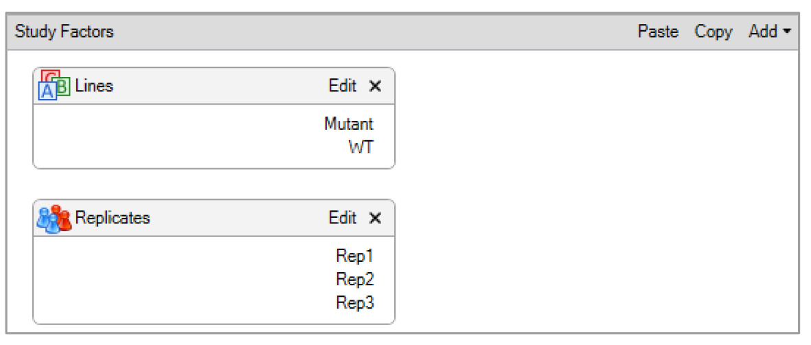
Figure 4. Design of study factors for the TMT-based quantitative proteomic analysis of the Arabidopsis proteome. The study factors show parameters, such as categorical factors, denoted as lines (upper box), and replicates (lower box), to create sample groups defined in the experiment.
6. On the Sample tab, specify the sample type as Control and/or Sample.
7. Open New Analysis and drag the sample file to the Analysis section.
8. Create the processing (see Figure 5A, B) and consensus workflow (see Figure 6A, B) in the Workflows tab by dragging and connecting nodes from the Workflow Nodes to the Workflow Tree.
Optional: Use our workflow.
Note: In the MSPepSearch node, select all four Arabidopsis spectral libraries (A, B, C, and D).
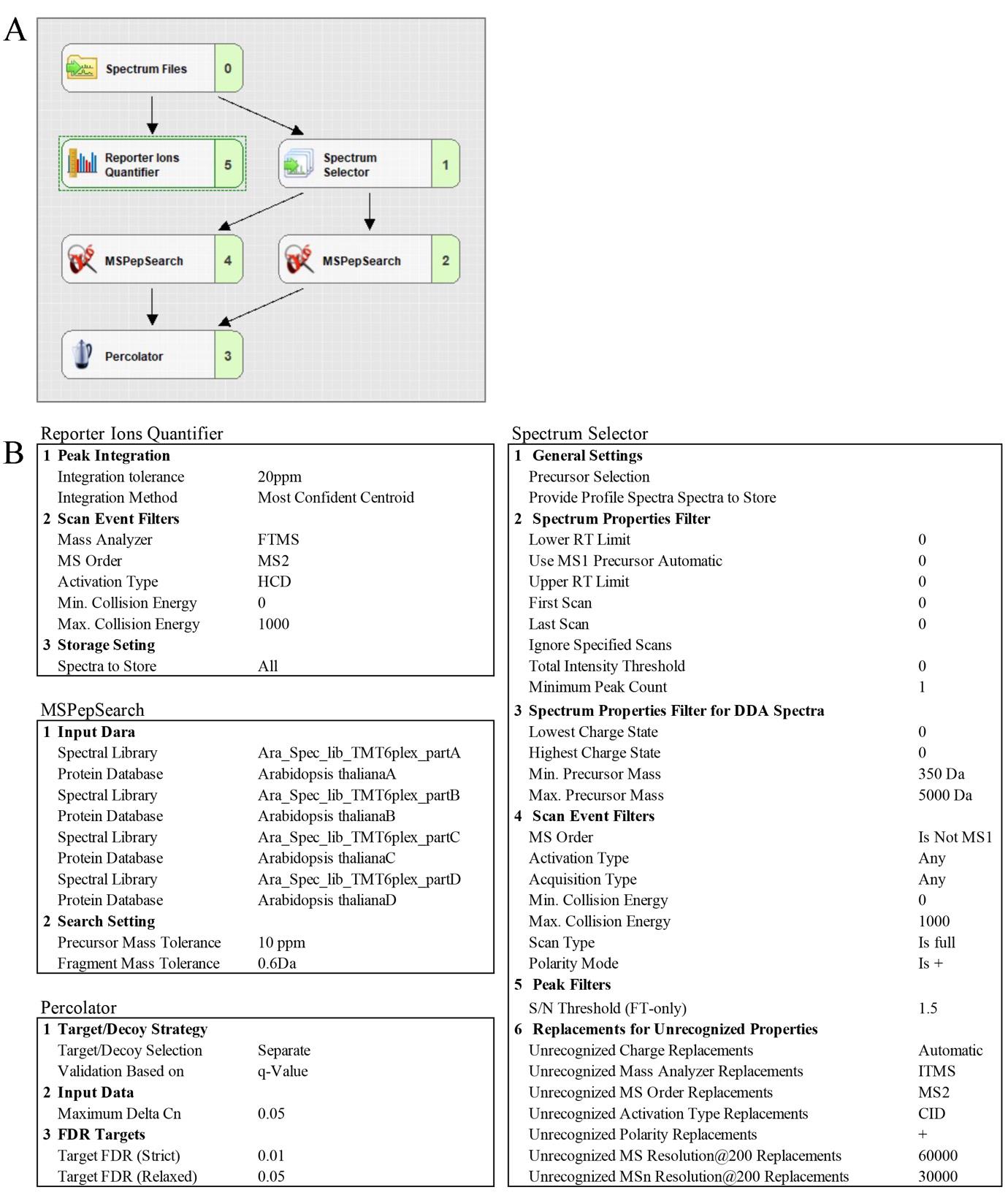
Figure 5. Proteome Discoverer setting for the TMT-based quantitative proteomic analysis of the Arabidopsis proteome. (A) Processing workflow. (B) Parameters for Report Ion Quantifier, Spectrum Selector, MSPepSearch, and Percolator nodes.
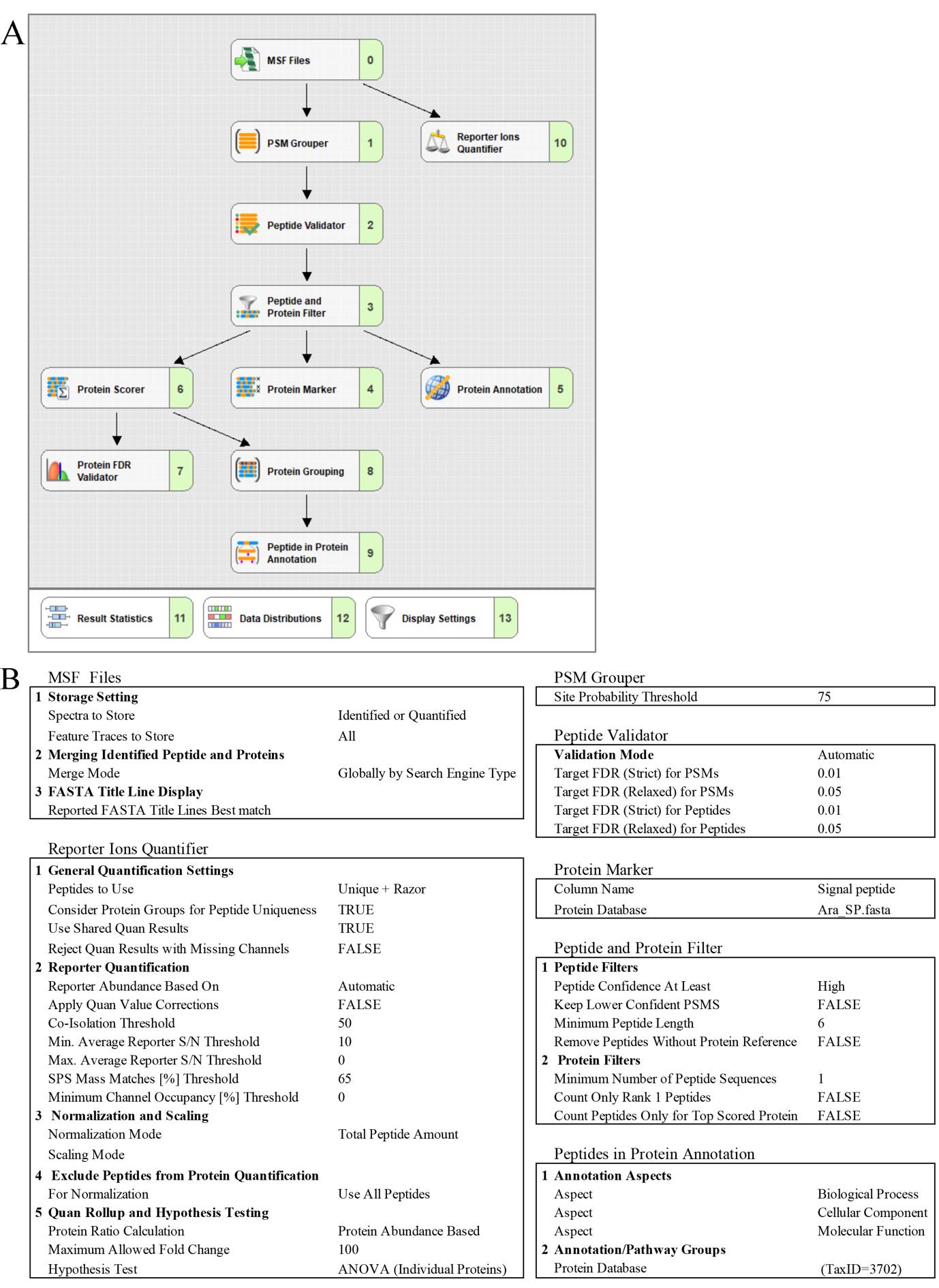
Figure 6. Proteome Discoverer setting for the TMT-based quantitative proteomic analysis of the Arabidopsis proteome. (A) Consensus workflow. (B) Parameters for MSF Files, Report Ions Quantifier, PSM Grouper, Peptide Validator, Protein Marker, Peptide and Protein Filter, and Peptides in Protein Annotation.
9. In the Grouping and Quantification tab, generate the Sample Groups by clicking the Study Variables (Files, Quan Channels, Lines, and Sample Type). In the example below, we used Lines to generate mutant/WT ratios with a nested design (see Figure 7).
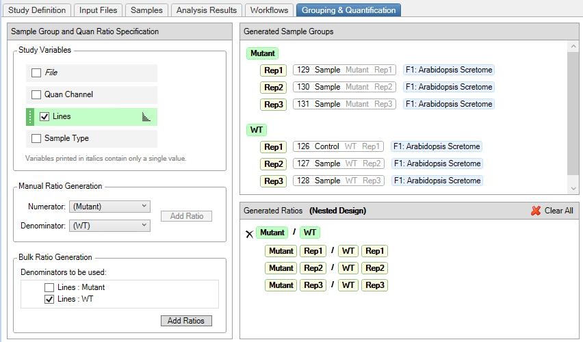
Figure 7. Proteome Discoverer setting for the grouping and quantification of Arabidopsis TMT-labeled peptides. Sample groups are generated by selecting the categorical factor (Lines), and mutants are ratioed against the WT to generate replicates in a nested design.
10. For the identification of secretory proteins in the conventional secretory pathway, download the Arabidopsis protein database with signal peptides, transmembrane domains, and ER retention signals from UniProt in FASTA format. Add the FASTA files in PD 3.0 by selecting FASTA files on the Administration start page. Use these files in the Protein Marker node to annotate the secretory proteins.
In our previous studies, we classified a secretory protein that contains a signal peptide and lacks a membrane anchor and ER retention signal [4].
General notes and troubleshooting
During the apoplast flush extraction from Arabidopsis leaves, caution is advised to minimize cell breakage and leakage throughout the process. Because intracellular protein leaking into the apoplast is inevitable, it is recommended that the contaminant background be below 1% and remain uniform across all samples.
To determine cytoplasmic contamination in the apoplast sample before mass spectrometry analysis, Rubisco can be detected by immunoblot analysis with anti-Rubisco antibodies, as described in Waghmare et al. [21]. If anti-Rubisco antibodies are not available, other cytoplasmic contaminants, such as malate dehydrogenase (MDH), 3 glucose-6-phosphate dehydrogenase (G6PDH), and glucose-6-phosphate (G-6-P) can be detected using commercially available assay kits [23].
In proteomics analysis, detection of Rubisco is unavoidable, as it is a highly abundant protein in plants and thus detectable even in highly pure apoplast samples. We recommend using different cytoplasm resident proteins as a measure of purity, including MALATE DEHYDROGENASE 1 (MDH, AT1G04410) and CATALASE 3 (CAT3, AT1G20620) as described before [23].
We recommend using at least two different approaches to evaluate apoplast sample purity. We suggest conducting a small aliquot of label-free mass spectrometry (see Sections C and E) to assess peptide preparation quality, considering budgetary constraints.
Validation of protocol
This protocol (or parts of it) were used and validated in following research articles:
• Waghmare et al. [21]. SYNTAXIN OF PLANTS 132 underpins secretion of cargoes associated with salicylic acid signalling and pathogen defense. Plant Physiology (Figures 1E–G, 2A–E, and 3A show data from TMT–MS analysis of Arabidopsis leaf apoplast secretome).
• Baena et al. [6]. SNARE SYP132 mediates divergent traffic of plasma membrane H+-ATPase AHA1 and antimicrobial PR1 during bacterial pathogenesis. Plant Physiology (Figure 4A–C shows apoplast flush extraction and analysis of antimicrobial secreted cargo using immunoblot).
Apoplast purity was determined by immunoblotting analysis of Rubisco heavy chain protein (∼53 kDa), a highly abundant cytoplasmic protein, compared with total leaf tissue lysate (estimated >99%).
TMT labeling efficiency ranged between 97% and 99% across all samples (>95% acceptable). The robustness and reproducibility of the method were validated through variability in experimental replicates using hierarchical clustering and principal component analysis (PCA). The abundance patterns of secretory cargoes in the controls and treatments/mutants were consistent within the sample groups, indicating alterations in protein abundances only between the two groups. TMT–MS quantification of secretory proteins in the mutants/treatments was verified by immunoblotting analysis targeting PR2 protein (∼34 kDa), a secretory cargo that responds to pathogen treatment in our experiment. The results from immunoblotting analysis agreed with the TMT–MS analysis.
Acknowledgments
This work was supported by grants from the Biotechnology and Biological Sciences Research Council (BB/X013383/1, BB/Y010272/1, BB/Z516788/1, BB/S017348/1, BB/S506734/1), Wellcome ISSF Excellence and Innovation Catalyst Funding (204820/Z/16/Z), The Leverhulme Trust (RPG-2024-397), and The Royal Society (University Research Fellowship UF150364, URF\R\211002) to R.K. This protocol was used in [6,21].
The following figures were created using BioRender: Graphical overview, BioRender.com/ MC28UQ1V5I.
Competing interests
The authors declare no conflicts of interest.
References
- Agrawal, G. K., Jwa, N. S., Lebrun, M. H., Job, D. and Rakwal, R. (2010). Plant secretome: unlocking secrets of the secreted proteins. Proteomics. 10(4): 799–827. https://doi.org/10.1002/pmic.200900514
- Tanveer, T., Shaheen, K., Parveen, S., Kazi, A. G. and Ahmad, P. (2014). Plant secretomics: identification, isolation, and biological significance under environmental stress. Plant Signal Behav. 9(8): e29426. https://doi.org/10.4161/psb.29426
- Ngara, R., Ramulifho, E., Movahedi, M., Shargie, N. G., Brown, A. P. and Chivasa, S. (2018). Identifying differentially expressed proteins in sorghum cell cultures exposed to osmotic stress. Sci Rep. 8(1): 8671. https://doi.org/10.1038/s41598-018-27003-1
- Waghmare, S., Lileikyte, E., Karnik, R., Goodman, J. K., Blatt, M. R. and Jones, A. M. (2018). SNAREs SYP121 and SYP122 Mediate the Secretion of Distinct Cargo Subsets. Plant Physiol. 178(4): 1679–1688. https://doi.org/10.1104/pp.18.00832
- Cheng, F. Y. and Williamson, J. D. (2010). Is there leaderless protein secretion in plants? Plant Signal Behav. 5(2): 129–131. https://doi.org/10.4161/psb.5.2.10304
- Baena, G., Xia, L., Waghmare, S. and Karnik, R. (2022). SNARE SYP132 mediates divergent traffic of plasma membrane H+-ATPase AHA1 and antimicrobial PR1 during bacterial pathogenesis. Plant Physiol. 189(3): 1639–1661. https://doi.org/10.1093/plphys/kiac149
- Baena, G., Xia, L., Waghmare, S., Yu, Z., Guo, Y., Blatt, M. R., Zhang, B. and Karnik, R. (2024). Arabidopsis SNARE SYP132 impacts on PIP2;1 trafficking and function in salinity stress. Plant J. 118(4): 1036–1053. https://doi.org/10.1111/tpj.16649
- Xia, L., Mar Marquès-Bueno, M., Bruce, C. G. and Karnik, R. (2019). Unusual Roles of Secretory SNARE SYP132 in Plasma Membrane H+-ATPase Traffic and Vegetative Plant Growth. Plant Physiol. 180(2): 837–858. https://doi.org/10.1104/pp.19.00266
- Hafidh, S., Potesil, D., Fila, J., Capkova, V., Zdrahal, Z. and Honys, D. (2016). Quantitative proteomics of the tobacco pollen tube secretome identifies novel pollen tube guidance proteins important for fertilization. Genome Biol. 17: 81. https://doi.org/10.1186/s13059-016-0928-x
- Goeminne, L. J. E., Gevaert, K. and Clement, L. (2018). Experimental design and data-analysis in label-free quantitative LC/MS proteomics: A tutorial with MSqRob. J Proteomics. 171: 23–36. https://doi.org/10.1016/j.jprot.2017.04.004
- Megger, D. A., Pott, L. L., Ahrens, M., Padden, J., Bracht, T., Kuhlmann, K., Eisenacher, M., Meyer, H. E. and Sitek, B. (2014). Comparison of label-free and label-based strategies for proteome analysis of hepatoma cell lines. Biochim Biophys Acta. 1844(5): 967–976. https://doi.org/10.1016/j.bbapap.2013.07.017
- Thompson, A., Schafer, J., Kuhn, K., Kienle, S., Schwarz, J., Schmidt, G., Neumann, T., Johnstone, R., Mohammed, A. K. and Hamon, C. (2003). Tandem mass tags: a novel quantification strategy for comparative analysis of complex protein mixtures by MS/MS. Anal Chem. 75(8): 1895–1904. https://doi.org/10.1021/ac0262560
- Thompson, A., Wolmer, N., Koncarevic, S., Selzer, S., Bohm, G., Legner, H., Schmid, P., Kienle, S., Penning, P., Hohle, C., et al. (2019). TMTpro: Design, Synthesis, and Initial Evaluation of a Proline-Based Isobaric 16-Plex Tandem Mass Tag Reagent Set. Anal Chem. 91(24): 15941–15950. https://doi.org/10.1021/acs.analchem.9b04474
- Zuniga, N. R., Frost, D. C., Kuhn, K., Shin, M., Whitehouse, R. L., Wei, T. Y., He, Y., Dawson, S. L., Pike, I., Bomgarden, R. D., et al. (2024). Achieving a 35-Plex Tandem Mass Tag Reagent Set through Deuterium Incorporation. J Proteome Res. 23(11): 5153–5165. https://doi.org/10.1021/acs.jproteome.4c00668
- Navarrete-Perea, J., Yu, Q., Gygi, S. P. and Paulo, J. A. (2018). Streamlined Tandem Mass Tag (SL-TMT) Protocol: An Efficient Strategy for Quantitative (Phospho)proteome Profiling Using Tandem Mass Tag-Synchronous Precursor Selection-MS3. J Proteome Res. 17(6): 2226–2236. https://doi.org/10.1021/acs.jproteome.8b00217
- Zecha, J., Satpathy, S., Kanashova, T., Avanessian, S. C., Kane, M. H., Clauser, K. R., Mertins, P., Carr, S. A. and Kuster, B. (2019). TMT Labeling for the Masses: A Robust and Cost-efficient, In-solution Labeling Approach. Mol Cell Proteomics. 18(7): 1468–1478. https://doi.org/10.1074/mcp.TIR119.001385
- Bachor, R., Waliczek, M., Stefanowicz, P. and Szewczuk, Z. (2019). Trends in the Design of New Isobaric Labeling Reagents for Quantitative Proteomics. Molecules. 24(4): 701. https://doi.org/10.3390/molecules24040701
- Martínez‐González, A. P., Ardila, H. D., Martínez‐Peralta, S. T., Melgarejo‐Muñoz, L. M., Castillejo‐Sánchez, M. A. and Jorrín‐Novo, J. V. (2018). What proteomic analysis of the apoplast tells us about plant–pathogen interactions. Plant Pathol. 67(8): 1647–1668. https://doi.org/10.1111/ppa.12893
- Deutsch, E. W. (2011). Tandem mass spectrometry spectral libraries and library searching. Methods Mol Biol. 696: 225–232. https://doi.org/10.1007/978-1-60761-987-1_13
- Zhang, H., Liu, P., Guo, T., Zhao, H., Bensaddek, D., Aebersold, R. and Xiong, L. (2019). Arabidopsis proteome and the mass spectral assay library. Sci Data. 6(1): 278. https://doi.org/10.1038/s41597-019-0294-0
- Waghmare, S., Xia, L., Ly, T. P., Xu, J., Farami, S., Burchmore, R., Blatt, M. R. and Karnik, R. (2025). SYNTAXIN OF PLANTS 132 underpins secretion of cargoes associated with salicylic acid signaling and pathogen defense. Plant Physiol. 197(1). e1093/plphys/kiae541. https://doi.org/10.1093/plphys/kiae541
- Wisniewski, J. R., Zougman, A., Nagaraj, N. and Mann, M. (2009). Universal sample preparation method for proteome analysis. Nat Methods. 6(5): 359–362. https://doi.org/10.1038/nmeth.1322.
- Alexandersson, E., Ali, A., Resjo, S. and Andreasson, E. (2013). Plant secretome proteomics. Front Plant Sci. 4: 9. https://doi.org/10.3389/fpls.2013.00009
Article Information
Publication history
Received: Jul 22, 2025
Accepted: Oct 8, 2025
Available online: Oct 21, 2025
Published: Nov 20, 2025
Copyright
© 2025 The Author(s); This is an open access article under the CC BY license (https://creativecommons.org/licenses/by/4.0/).
How to cite
Readers should cite both the Bio-protocol article and the original research article where this protocol was used:
- Waghmare, S., Xia, L., McGill, S., Burchmore, R. and Karnik, R. (2025). Quantitative Analysis of the Arabidopsis Leaf Secretory Proteome via TMT-Based Mass Spectrometry. Bio-protocol 15(22): e5508. DOI: 10.21769/BioProtoc.5508.
- Waghmare, S., Xia, L., Ly, T. P., Xu, J., Farami, S., Burchmore, R., Blatt, M. R. and Karnik, R. (2025). SYNTAXIN OF PLANTS 132 underpins secretion of cargoes associated with salicylic acid signaling and pathogen defense. Plant Physiol. 197(1). e1093/plphys/kiae541. https://doi.org/10.1093/plphys/kiae541
Category
Plant Science > Plant biochemistry > Protein
Plant Science > Plant molecular biology > Protein
Systems Biology > Proteomics
Do you have any questions about this protocol?
Post your question to gather feedback from the community. We will also invite the authors of this article to respond.