- Protocols

- Articles and Issues
- For Authors
- About
- Become a Reviewer

In Silico Prediction and In Vitro Validation of Bacterial Interactions in the Plant Rhizosphere Using a Synthetic Bacterial Community
Published: Vol 15, Iss 21, Nov 5, 2025 DOI: 10.21769/BioProtoc.5496 Views: 1656
Reviewed by: Shweta PanchalPayton Tung-On YauAnonymous reviewer(s)
Original research article
The authors used this protocol in:

Oct 2025

Protocol Collections
Comprehensive collections of detailed, peer-reviewed protocols focusing on specific topics


Related protocols

Abstract
The rhizosphere, a 2–10 mm region surrounding the root surface, is colonized by numerous microorganisms, known as the rhizosphere microbiome. These microorganisms interact with each other, leading to emergent properties that affect plant fitness. Mapping these interactions is crucial to understanding microbial ecology in the rhizosphere and predicting and manipulating plant health. However, current methods do not capture the chemistry of the rhizosphere environment, and common plant–microbe interaction study setups do not map bacterial interactions in this niche. Additionally, studying bacterial interactions may require the creation of transgenic bacterial lines with markers for antibiotic resistance/fluorescent probes and even isotope labeling. Here, we describe a protocol for both in silico prediction and in vitro validation of bacterial interactions that closely recapitulate the major chemical constituents of the rhizosphere environment using a widely used Murashige & Skoog (MS)-based gnotobiotic plant growth system. We use the auto-fluorescent Pseudomonas, abundantly found in the rhizosphere, to estimate their interactions with other strains, thereby avoiding the need for the creation of transgenic bacterial strains. By combining artificial root exudate medium, plant cultivation medium, and a synthetic bacterial community (SynCom), we first simulate their interactions using genome-scale metabolic models (GSMMs) and then validate these interactions in vitro, using growth assays. We show that the GSMM-predicted interaction scores correlate moderately, yet significantly, with their in vitro validation. Given the complexity of interactions among rhizosphere microbiome members, this reproducible and efficient protocol will allow confident mapping of interactions of fluorescent Pseudomonas with other bacterial strains within the rhizosphere microbiome.
Key features
• This method builds upon the widely used MS-based gnotobiotic system for growing plants and a synthetic bacterial community (SynCom) for plant–microbe interaction studies.
• It considers the chemical composition of plant growth media (MS) and root exudates to map bacterial interactions.
• It provides a method to both predict and validate interactions of fluorescent Pseudomonas with other strains within a SynCom.
• This method is scalable for any bacterial pair with distinguishing markers (e.g., fluorescence, antibiotic resistance).
Keywords: Microbial interactionsGraphical overview
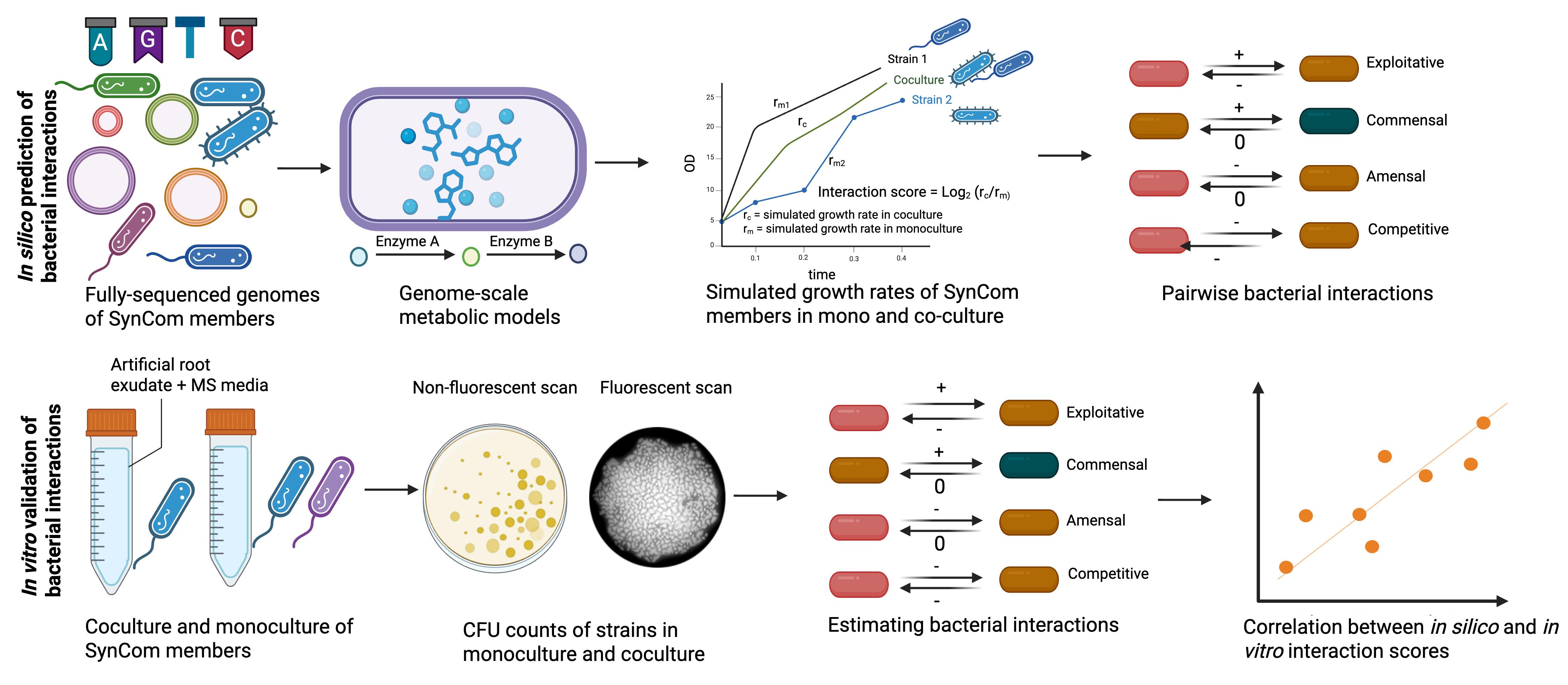
Workflow for in silico prediction and in vitro validation of bacterial interactions. Genome sequences of synthetic bacterial community (SynCom) members are used to infer their genome-scale metabolic models (GSMMs). These models are then used to simulate growth in monoculture and in coculture with the interacting strains in chemically defined artificial root exudates + MS media. This same media is later used to calculate interaction scores and classify them in ecological terms through colony-forming unit (CFU) counts, in vitro. Individual strains are grown (same media as we used for in silico prediction) in monoculture and in coculture with interacting strains for 24 h, with an initial OD of 0.02 for each of the strains. Following their growth, cultures are serially diluted in King’s B agar media to estimate the count of fluorescent Pseudomonas and the other strain using fluorescent and non-fluorescent scans. CFU counts are estimated with ImageJ and subsequently used to calculate their interaction scores. In this protocol, the fluorescent Pseudomonas sp. 6A2 is used as an example to estimate its interaction with other members of the SynCom. Any other marker, e.g., antibiotic resistance, could be used for estimating interaction scores.
Background
Plants host phylogenetically diverse microbial communities (microbiomes) across their niches—the root, shoot, and rhizosphere [1,2]. Members of the microbiome can influence plant fitness, either individually or through their interaction with other microbial members, leading to emergent properties [3]. Mapping these interactions is therefore important but remains a challenge. The introduction of synthetic bacterial communities has greatly simplified our ability to deconstruct these complex microbe–microbe interactions.
Pairwise bacterial interactions could be mapped experimentally and have been shown to infer complex ecological dynamics within multi-species communities [4,5]. In parallel, advances in computational approaches have greatly enhanced our ability to predict these interactions. Using genome-scale metabolic models (GSMMs), researchers have mapped the microbial interactions in diverse ecosystems, including the human gut and the phyllosphere [6,7]. This approach is more accurate than correlation-based approaches, enabling the prediction of numerous possible interactions within a microbial community, which otherwise is tedious to perform experimentally [8]. However, it is crucial to validate them experimentally for better confidence in these computational predictions.
Plate-based systems are traditionally used to study plant–microbe interactions in a gnotobiotic setup [9]. Microbes added to the plant roots rely on root exudates for survival and colonization. Additionally, the chemistry of the root exudates could greatly influence bacterial interactions in the rhizosphere. The chemical environment in these systems greatly influence the outcome of plant–microbe and microbe–microbe interactions. Although a few studies have attempted to map bacterial interactions within the plant microbiome, the chemical environment of Murashige & Skoog (MS)-based gnotobiotic systems and the effects of plant-derived chemicals are often ignored [10]. In this protocol, we present both computational and experimental validation of bacterial interactions, considering the chemistry of root exudates and the MS-based gnotobiotic system. We use a fluorescent pseudomonad species within our synthetic bacterial community (SynCom) to differentiate its colony-forming unit (CFU) counts from other bacterial species in coculture. Since fluorescent pseudomonads are a majorly abundant bacterial species in the rhizosphere, this protocol will be useful in future studies [11]. Even though the chemical composition of root exudates is simplified, our computational prediction and experimental validation correlate with each other. This method for mapping bacterial interactions in the rhizosphere can be extended to other gnotobiotic plant-growth systems and plant niches.
Materials and reagents
Biological materials
1. The following 17 bacterial strains were used to study their interactions with the fluorescent strain Pseudomonas sp. 6A2: (i) Paenibacillus sp. 8E4, (ii) Pseudomonas sp. 9F3, (iii) Mycoplana sp. P31D, (iv) Brevundimonas sp. 9B2, (v) Candidimonas sp. 4C, (vi) Achromobacter sp. 1A1, (vii) Xanthomonas sp. 3C2, (viii) Atlantibacter sp. P33G, (ix) Lysinibacillus sp. 3C1, (x) Bhargaveae sp. 9B1, (xi) Bacillus sp. 8A2, (xii) Priestia sp. 7F21, (xiii) Corynebacterium sp. 10B2, (xiv) Agromyces sp. 9E2, (xv) Cellulosimicrobium sp. 8E1, (xvi) Streptomyces sp. P32B1, (xvii) Streptomyces sp. 6A1
In this protocol, this collection of 17 strains is named SynCom18.
All the above strains can be grown to saturation within 24 h in Luria broth (LB) media. Store the strains in 25% glycerol at -80 °C for long-term storage. While growing the strains for monoculture/coculture experiments, streak them as single colonies in LB agar plates.
Note: The inherent fluorescence of Pseudomonas sp. 6A2 is used as a distinguishing feature for CFU counts of individual strains in coculture. This method, therefore, requires distinguishing markers of bacterial strains to estimate CFU in coculture with other bacterial strains. This could be colony morphology, fluorescence, or antibiotic resistance.
Reagents
1. Glucose (Sigma, CAS number: 50-99-7)
2. Fructose (Sigma, CAS number: 57-48-7)
3. Sucrose (Sigma, CAS number: 57-50-1)
4. Succinic acid (Sigma, CAS number: 110-15-6)
5. L-Alanine (Sigma, CAS number: 56-41-7)
6. L-Serine (Sigma, CAS number: 56-45-1)
7. Citric acid (Sigma, CAS number: 77-92-9)
8. Sodium lactate (Sigma, CAS number: 72-17-3)
9. Glycine (Sigma, CAS number: 56-40-6)
10. Nicotinic acid (Sigma, CAS number: 59-67-6)
11. Pyridoxine HCl (Sigma, CAS number: 58-56-0)
12. Thiamine HCl (Sigma, CAS number: 67-03-9)
13. MS (Sigma, catalog number: M5519)
14. MES hydrate (Sigma, CAS number: 1266615-59-1)
15. Glycerol (Sigma, CAS number: 56-81-5)
16. Luria broth (Sigma, catalog number: 146813)
17. Bacto agar (Sigma, CAS number: 9002-18-0)
18. King agar B (Sigma, catalog number: 60786)
19. Magnesium chloride (MgCl2) (Sigma, catalog number: M8266)
Solutions
1. Artificial root exudates (ARE), 10× stock (see Recipes)
2. Vitamin stock (1,000×) (see Recipes)
3. MS media (2× stock) (see Recipes)
4. Luria broth (LB)
Recipes
Note: Prepare all solutions in a sterile laminar hood and store in sterile glass bottles.
1. Artificial root exudates (ARE), 10× stock
| Reagent | Final concentration | Quantity or volume |
|---|---|---|
| Glucose | 16.4 g/L | 100 mL |
| Fructose | 16.4 g/L | 100 mL |
| Sucrose | 8.4 g/L | 100 mL |
| Succinic acid | 9.2 g/L | 10 mL |
| Alanine | 8 g/L | 10 mL |
| Serine | 9.6 g/L | 10 mL |
| Citric acid | 3.2 g/L | 10 mL |
| Sodium lactate | 6.4 g/L | 10 mL |
ARE recipe was adapted from Getzke et al. [12].
2. Vitamin stock (1,000×)
| Reagent | Final concentration | Quantity or volume |
|---|---|---|
| Glycine | 2,000 mg/L | 10 mL |
| Nicotinic acid | 500 mg/L | 10 mL |
| Pyridoxine HCl | 500 mg/L | 10 mL |
| Thiamine HCl | 100 mg/L | 10 mL |
Can be stored at 4 °C for approximately 1 month.
3. MS media (2× stock)
Prepare a 2× stock of MS media by adding 8.8 g of MS salt in 1 L of distilled water with 1 g of MES hydrate. MS media can be stored at 4 °C for approximately 1 month after autoclaving.
Prepare 100 mL of ARE + vitamin stock + MS media by adding 50 mL of 2× MS stock to 10 mL of ARE 10× stock and 100 μL of 1,000× vitamin stock. Filter-sterilize ARE and vitamin stock using a 0.22 μm membrane before adding to MS media. Autoclave (121 °C for 20 min) and cool down the MS media before adding to ARE and vitamin solution. Set the pH of the total mixed solution to 7 before use.
Laboratory supplies
1. 50 and 15 mL Falcon tubes (NuncTM Conical Sterile Polypropylene Centrifuge Tubes) (Thermo Scientific, catalog number: 12-565-269)
2. 1.5 and 2 mL tubes (Safe-Lock Tubes 1.5 mL, Microtube) (Eppendorf, catalog number: 05-402-27)
3. L-shaped Spreader (L-Shape, sterile) (Sigma, catalog number: HS8171B)
4. Petri plates (NuncTM Petri dishes) (Thermo Scientific, catalog number: 08-757-099)
5. Inoculation loops (Thermo Scientific, Disposable Calibrated Inoculating Loops, catalog number: R501400)
6. Pipette tips (1–10 μL, 20–200 μL, and 100–1,000 μL) (FinntipTM Pipette Tips, catalog number: 9401115)
7. Pipettes (1–10 μL, 20–200 μL, and 100–1,000 μL) (PIPETMAN 4-Pipette Kit, catalog number: F167360)
Equipment
1. Plate reader (Agilent BioTek Synergy H1 Multimode Reader)
2. Gel scanner 2 (GelDoc Go Gel Imaging System with Image Lab Touch Software, catalog number: 12009077)
Software and datasets
1. Image J (v1.54p freely available) [13]
2. R (v4.4.1 freely available)
3. Python (v3.8 freely available)
4. MEMOTE (v0.14.0) (python-based application and freely available) [14]
5. gapseq (v1.4.0) (R-based application and freely available) [15]
All data and code have been deposited to GitHub: https://github.com/arijitnus/Bio-protocol/ (access date, 05/16/2025).
Procedure
Part I: In silico prediction of bacterial interactions in the rhizosphere using genome-scale metabolic models (GSMMs)
A. Reconstruction of genome-scale metabolic models of bacterial members within a SynCom
We used the SynCom 18 (see Biological materials) to generate genome-scale metabolic models (GSMMs) of individual bacterial members using the tool gapseq (see Software and datasets). GSMMs are reconstructed in silico, in three distinct steps: (i) metabolic pathways and transporters prediction, (ii) draft reconstruction of GSMMs, and (iii) multi-step gap-filling. A basic proficiency in shell scripting is required for these steps. The detailed steps are described below:
1. Installation of gapseq
gapseq can be installed with miniconda in a Linux-based system. To install gapseq, create a conda environment using the command listed here: https://gapseq.readthedocs.io/en/latest/install.html.
Note: cplexsolver should be installed to enable seamless simulation. Further details for the installation of gapseq can be found in the above link. A basic proficiency in shell scripting is required for running gapseq.
Use the following code as an example to install gapseq (comments are provided following a #)
conda create -c conda-forge -c bioconda -n gapseq gapseq# creates a conda environment gapseq and installs the gapseq tool within that environmentconda activate gapseq# This command activates the gapseq environment within conda. Always activate the environment before starting to code2. Prediction of transporters and pathways
Following the installation of gapseq, run the following command to predict the transporters and pathways within the bacterial genomes. For example, run the following command to predict all transporters and pathways within a bacterial genome (filename: bac.fna). All bacterial genome sequences can be found in File S1.
./gapseq find -p all bac.fna # predict the pathways within a bacterial genome. Use this command within the folder where bac.fna file is placed./gapseq find-transport bac.fna #predicts all the transporters within a bacterial genomeAlternatively, both transporters and pathways can be predicted with a single line of command:
./gapseq doall bac.fnaThe following output files are generated in this step:
(i) Pathways.tbl, (ii) Reactions.tbl, and (iii) Transporter.tbl. These files will have the prefix based on the name of the input bacterial strain.
The detailed codes are provided in https://github.com/arijitnus/Bio-protocol/ within the In silico prediction folder > model reconstruction. For example, model reconstruction for the 3C1 genome can be performed using the following command:
#1. Predict transporters, reactions, and all pathways./gapseq find -p all 3C2.fna # [code for predicting all reactions and pathways in a genome]./gapseq find-transport 3C2.fna # [code for predicting all transporters in a genome]./gapseq draft -r 9B2-all-Reactions.tbl -t 9B2-Transporter.tbl -p 9B2-all-Pathways.tbl -c 9B2.fna -u 200 -l 100 # [code for draft model preparation]./gapseq fill -m 9B2-draft.RDS -c 9B2-rxnWeights.RDS -g 9B2-rxnXgenes.RDS -n dat/media/ARE_MS_Vit.csv -b 100 # [code for gapfilling models]Input genome sequence of SynCom18 is provided in Zenodo: https://zenodo.org/records/16929714. Download the genomes from the above link and place them in a folder.
3. Draft network reconstruction and gap-filling
A novel Linear Programming (LP)-based gap-filling algorithm is used in ‘gapseq’ to enable biomass production in a given medium. Flux-balance analyses (FBA) are used for optimization.
Draft model reconstruction can be performed using the following command:
./gapseq draft -r bac-Reactions.tbl -t bac-Transporter.tbl -p bac-all-Pathways.tbl -c bac.fna.gz
# This command creates a draft metabolic model based on the input genome sequence. The input files are taken from step 2.
There are four output files from this step: (i) rxnWeights.RDS, (ii) rxnXgenes.RDS, (iii) draft.RDS, and (iv) draft.xml. The draft models are provided in both .RDS and .xml extension.
The detailed codes are provided in https://github.com/arijitnus/Bio-protocol/ within the In silico prediction folder > model reconstruction. Input files are the genome sequences of SynCom18.
Next, the draft models are fully reconstructed using gap-fill step. Use the following code as an example:
./gapseq fill -m -draft.RDS -n ARE_MS.csv -c -rxnWeights.RDS -g -rxnXgenes.RDS -b 100#The above command creates a gap-filled model from the input files in the draft model reconstruction step. The media composition can be found in https://github.com/arijitnus/Bio-protocol/ In silico prediction folder > ARE_MS_Vit.csv file.
The detailed codes are provided in https://github.com/arijitnus/Bio-protocol/ within the In silico prediction folder > model reconstruction, and input files can be found as In silico prediction folder > draft_models.zip.
4. Quality check using MEMOTE
Following reconstruction and gap-filling, check the quality of the GSMMs using the MEMOTE tool [12]. A basic level of Python skill is required to run MEMOTE on a local machine. Below is a snippet of the basic Python code required to calculate the quality score of GSMMs of a bacterial strain (bacteria1):
import memotememote report snapshot bacteria1.xmlThe above code takes as input the GSMM of bacteria1, which is an output from step 3. In place of bacteria1, use the input genome sequences for SynCom18 members. Use the gapfilled .xml file of GSMM. For a detailed instruction on the installation of MEMOTE, refer to the following document: https://github.com/opencobra/memote.
The MEMOTE output for all of the strains is accessible as HTML files in the following link: https://github.com/arijitnus/Bio-protocol/ within the In silico prediction folder MEMOTE_SynCom18.zip file.
Note that the overall percentage of score is considered for estimating the quality of the models (Table 1). The cutoff scores can be standardized from similar studies or GSMMs of similar bacterial strains. In our case, a MEMOTE score above 75% is considered for further analyses, based on our observation from the study by Schäfer et al. [6].
Table 1. MEMOTE score of the metabolic models of the SynCom18 members
| Strain | Overall score in MEMOTE |
|---|---|
| 1A1 | 78% |
| 8E4 | 60% |
| 3C1 | 77% |
| 3C2 | 77% |
| 4C | 77% |
| 6A1 | 77% |
| 6A2 | 77% |
| 8A2 | 77% |
| 8E1 | 77% |
| 9B1 | 77% |
| 9B2 | 77% |
| 9E2 | 77% |
| 9F3 | 77% |
| 10B2 | 77% |
| P32B1 | 77% |
| P33G | 77% |
| P31D | 77% |
| 7F21 | 61% |
Note: 8E4 and 7F21 had a poor-quality score and, therefore, were excluded from estimating bacterial interactions of these strains with others.
B. Simulating growth rates of bacterial members within a SynCom
Simulate the growth of individual bacterial strains and their coculture using the BacArena package in R [14]. Depending on the number of bacterial strains and their coculture, the system should be decided. For example, within an 18-membered SynCom, there are a total of 18C2 = 153 bacterial pairs of simulations required (the total number of pairs is calculated using the formula nC2, where n is the total number of bacterial strains, and 2 indicates pairwise combination). Therefore, the number of cocultures increases drastically with an increasing number of bacterial strains. In that case, use a high-performance computing (HPC) cluster.
Note that we have used 16 bacterial strains for calculating the interaction scores, since two bacterial strains Paenibacillus sp. 8E4 and Priestia sp. 7F21 did not meet the quality threshold in MEMOTE (Table 1).
Here, an example is provided for bacterial coculture and monoculture using two strains:
1. Simulating growth rates of individual bacterial strains
CRITICAL: The cplexsolver must be installed and tested before proceeding with this step. More details on the use and installation of cplexsolver can be found at https://www.ibm.com/products/ilog-cplex-optimization-studio/cplex-optimizer.
The R code is provided below, and an explanation for each line is provided with comments using ‘#’:
library(sybil) #loading librarylibrary(BacArena) #loading librarylibrary(parallel) #loading libraryrunSim <- function(i) { # params save_name <- 'Achromo_25h' # Name of the file as how it is saved arena_n <- 50 arena_m <- 50 time <- 25 initial_bacteria <- 2 sybil::SYBIL_SETTINGS("SOLVER","cplexAPI") bac1 <- BacArena::Bac((bac1), limit_growth=F, setAllExInf=T) arena <- BacArena::Arena(n=arena_n, m=arena_m, stir=F) arena <- BacArena::addOrg(arena, bac1, amount=initial_bacteria) arena <- BacArena::addSubs(arena, smax=1, unit='mM', mediac=paste0('EX_', media$compounds, '_e0')) # Begin the Simulation sim <- BacArena::simEnv(arena, time=time, diff_par = T, cl_size=3, sec_obj = 'mtf') saveRDS(sim, paste0(save_name, '_', i, '.RDS'))} # This function simulates the growth of bacterial strain in three replicates for 25hrs. The results are stored in ‘Achromo_25h_1.RDS’, ‘Achromo_25h_2.RDS’, and ‘Achromo_25h_3.RDS’.bac1 <- readRDS('Achromobacter.RDS') # Reads the GSMM output from gapfilling and reconstruction step for bacteria (here ‘Achromobacter.RDS’)bac1@mod_desc <- "Achromobacter" #description of the bacteriamedia <- read.csv('custom_MS_media_ARE.csv') #MS and ARE media for where we simulate the growth.replicates <- 3 # Three replicates of the growth simulationncores <- 3 # number of cores of the computing machine to usecl <- makeCluster(ncores,type="PSOCK")clusterExport(cl,c('bac1','media'))result <- parLapply(cl, 1:replicates, runSim)stopCluster(cl)print(result)2. Simulating growth rates of the coculture of a bacterial pair
The R code for simulating growth rates of all possible pairwise combinations for a number of bacteria is provided below:
library(sybil)library(BacArena)library(parallel)# Function to run simulation for a pair of bacteriarunSim <- function(bac1, bac2, i) { # params save_name <- paste0(bac1@mod_desc, '_', bac2@mod_desc, '_25h') # Updated save_name arena_n <- 50 # size of the arena n*m arena_m <- 50 time <- 25 initial_bacteria <- 2 sybil::SYBIL_SETTINGS("SOLVER","cplexAPI") bac1 <- BacArena::Bac(bac1, limit_growth=F, setAllExInf=T) bac2 <- BacArena::Bac(bac2, limit_growth=F, setAllExInf=T) arena <- BacArena::Arena(n=arena_n, m=arena_m, stir=F) arena <- BacArena::addOrg(arena, bac1, amount=initial_bacteria) arena <- BacArena::addOrg(arena, bac2, amount=initial_bacteria) arena <- BacArena::addSubs(arena, smax=1, unit='mM', mediac=paste0('EX_', media$compounds, '_e0')) # Begin the Simulation sim <- BacArena::simEnv(arena, time=time, diff_par = T, cl_size=5, sec_obj = 'mtf') saveRDS(sim, paste0(save_name, '_', i, '.RDS'))}# Read bacteria files from folderbacteria_folder <- "/Users/arijitmukherjee/Downloads/all_GMMs/"bacteria_files <- list.files(bacteria_folder, pattern = "\\.RDS$", full.names = TRUE)# Create all pairwise combinationsbacteria_combinations <- combn(bacteria_files, 2, simplify = TRUE)bacteria_combinationsmedia<-read.csv('/export2/home/arijit/bacarena/custom_MS_media_ARE.csv')# Set up parallel processingreplicates <- 3 # number of replicates to run in parallelncores <- 5cl <- makeCluster(ncores,type="PSOCK")clusterExport(cl, c('media', 'runSim','bacteria_combinations'))bac1<-readRDS(bacteria_combinations[1, i])bac2<-readRDS(bacteria_combinations[2, i])bac1@mod_name# Run simulations for each combination in parallelresult <- parLapply(cl, 1:ncol(bacteria_combinations), function(i) { bac1 <- readRDS(bacteria_combinations[1, i]) bac2 <- readRDS(bacteria_combinations[2, i]) runSim(bac1, bac2, i)})The detailed codes for monoculture and coculture can be found at https://github.com/arijitnus/Bio-protocol/ within the In silico prediction folder > monoculture.R and coculture_all_comb (1).R, respectively. The output files from simulation of monoculture and coculture are .RDS files, which are subsequently used for estimating interaction scores among the bacterial pairs.
C. Estimating interaction scores within a bacterial pair
From the above outputs in (B) and (C), extract the growth rates of individual bacterial members in monoculture (rm) and coculture (rc). Essentially, extract the number of bacterial cells with time and then use the R package growthcurver to extract the growth parameters, including the growth rates (rc and rm). The following code provides a detailed code for extracting growth rates from all SynCom18:
# List all bacteria nameslibrary(BacArena)library(sybil)library(ggplot2)library(dplyr)bacteria_names <- c("Atlanti", "Achromo", "Agromyces","Bacillus",
"Bhargavaea","Brevundimonas","Cellulosimicrobium",
"Corynebacterium","Lysinibacillus","Mycoplana",
"Paenibacillus","Priestia","Pseudomonas",
"Pseudomonas_guariconensis","Pusillimonas",
"Stenotrophomonas","Streptomyces","Streptomyces_griseofuscus") # Add all 18 bacteria names
# Initialize an empty list to store dataframesall_data <- list()# Loop through each bacteria and replicatefor (bacteria in bacteria_names) { for (replicate in 1:3) { # Create the file name file_name <- paste0(bacteria, "_25h_", replicate, ".RDS") # Read the .RDS file p <- readRDS(file_name) q <- plotGrowthCurve(p) data<-q$data # Extract the data data$bacteria <- bacteria data$replicate <- replicate # Append the dataframe to the list all_data[[length(all_data) + 1]] <- data }}# Merge all dataframes into onefinal_dataframe <- do.call(rbind, all_data)write.table(final_dataframe,'final_df.tsv',sep = "\t")# Print or use the final_dataframe as neededprint(final_dataframe)dim(final_dataframe)averaged_df <- final_dataframe %>% group_by(bacteria,time) %>% summarise(avg_value = mean(value))averaged_dfwrite.table(averaged_df,"averaged_df.tsv",sep = "\t")#calculate growth params for all strains using these packageslibrary(dplyr)library(reshape2)library(ggplot2)library(growthcurver)library(purrr)library(readxl)library(tidyr)#The above commands loads all librariesspread_avg_df<-spread(averaged_df,key = bacteria,value = avg_value)spread_avg_dfspread_avg_df$Time<-spread_avg_df$time*60names(spread_avg_df)spread_avg_df<-spread_avg_df[,-1]#filter the data for 30hrs=1800 mins for logistic growth curve This is based on#information of plotting the data previouslygrowth.values.plate <- SummarizeGrowthByPlate(spread_avg_df)growth.values.platewrite.table(growth.values.plate,"growth-values-plate.tsv",sep = "\t")This can also be found in https://github.com/arijitnus/Bio-protocol/ within the In silico prediction folder > growth_curve_params.R (for monoculture/coculture of all 16 bacterial strains).
Next, use the following R code to calculate the interaction scores for each of the bacterial pairs from the 18 members SynCom:
rds_files <- list.files(pattern = "\\.RDS$")#List all .RDS model files of the SynCom strainsrds_filesdata_list <- list()library(BacArena)for (file_name in rds_files) { # Read the .RDS file p <- readRDS(file_name) # Assuming plotGrowthCurve and q$data are correct based on your code data <- plotGrowthCurve(p)[[1]]$data # Store the data with the specified name data_name<-paste(unique(data$species),collapse = "_") assign(data_name, data) # Add the data to the list data_list[[data_name]] <- data}length(data_list)#install.packages("tidyverse")library(tidyverse)library(growthcurver)result_list<-list()# Loop through each dataframe in the listfor (i in seq_along(data_list)) { # Spread the dataframe spread_df <- spread(data_list[[i]], key = species, value = value) spread_df$Time <- spread_df$time * 60 spread_df <- spread_df[, -c(1, 2)] # Summarize growth by plate growth.values.plate <- SummarizeGrowthByPlate(spread_df) # Store the result in the list result_list[[paste("result_", i, sep = "")]] <- growth.values.plate}saveRDS(result_list,'growth_params_coculture_revised.RDS')library(dplyr)library(tidyr)merged_data <- bind_rows(result_list, .id = "source_df")head(merged_data)write.table(merged_data,'coculture_all_data_revised.tsv',sep = "\t")monoculture_growth_rate <- read.table(‘monoculture_growth_rates.tsv’, header = TRUE, stringsAsFactors = FALSE) #Read in the monoculture growth rates of individual bacterial strainsmerged_data2 <- merged_data %>% left_join(monoculture_growth_rate, by = "sample") %>% mutate(interaction_score =log2(r/rm))write.table(merged_data2,'interaction_scores.tsv',sep = "\t") #writes out the interaction scores in the working directoryThe above code can also be found at https://github.com/arijitnus/Bio-protocol/ within the In silico prediction folder > Interactionscore_calc.R
The above code provides a matrix of interaction scores for all possible pairwise combinations within the SynCom18. The interaction scores for a bacterial pair (strain A and B) are calculated using the following formula:
Interaction score of strain A = Log2 (rcA/rmA)
Interaction score of strain B = Log2 (rcB/rmB)
Here, rcA and rmA refer to the growth rates of strain A in monoculture and coculture (with strain B), respectively.
The results from pairwise interactions of 6A2 and other bacterial strains are shown in Figure 1.
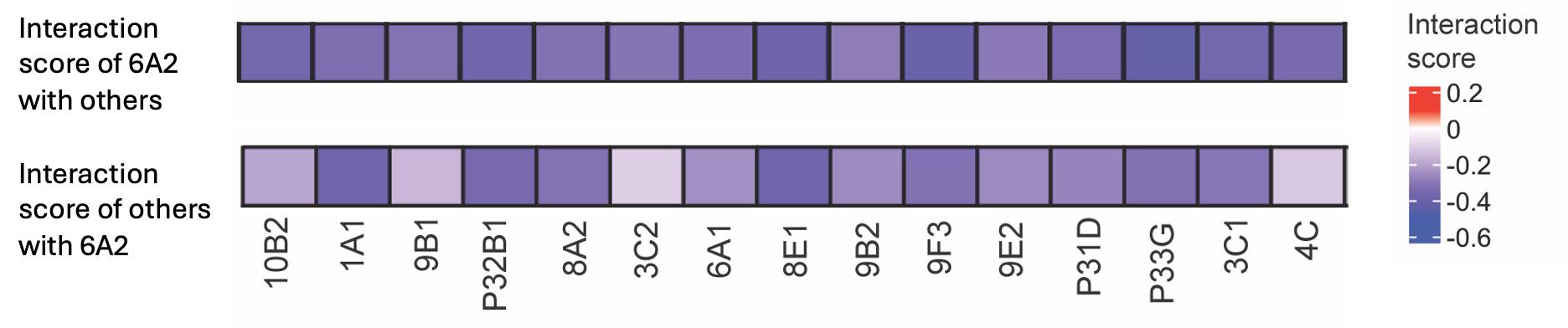
Figure 1. Heatmap showing the in silico predicted interaction scores among Pseudomonas sp. 6A2 and other members of the SynCom. Colors indicate the interaction scores predicted from their simulated growth rates in monoculture and coculture. Two separate heatmaps are shown: the top panel for other strains with 6A2 and the bottom panel for 6A2 with other strains. This figure was prepared using the ComplexHeatmap package in R (v 4.4.1).
Part II: In vitro validation of bacterial interaction
A. Culturing bacterial strains in monoculture and in coculture
1. Culture bacterial strains overnight in generic microbiological media (e.g., LB media) by inoculating single colonies streaked in plates.
2. In the morning, centrifuge the overnight-grown culture at 8,000× g for 5 min.
3. Discard the supernatant and wash twice using sterile 10 mM MgCl2 by mixing the pellet, spinning down, and discarding the supernatant.
PAUSE POINT: The washed bacterial pellets can be stored for 2 h on ice.
4. Finally, reconstitute the bacterial pellet in 5 mL of 10 mM MgCl2 and mix the bacterial cells by pipetting.
5. Measure the O.D. of bacterial culture with an appropriate control (10 mM MgCl2 without any bacteria).
6. Calculate the volume required for a final O.D. of 0.02 in 5 mL for each of the strains. For example, if the initial O.D. of an overnight-grown bacterial culture is 1.1, then (5000 × 0.02)/1.1 ~91 μL of this bacterial strain should be added to ~4,910 μL of culture medium.
7. Now, for each bacterial pair, consider three different conditions: (i) monoculture of strain A, (ii) monoculture of strain B, and (iii) coculture of strains A and B. For (i) and (ii), add the volume of strain A or B calculated in step A6 to the ARE + MS media. For (iii), add the required volumes of strain A and B to a final volume of 5 mL.
Note: Aspirate out the volume of strains A or B to be added from the culture tubes before adding the bacterial strains. If considering 3 replicates per condition, prepare three different culture tubes accordingly.
8. Place the tubes in a 30 °C shaking incubator at 200 rpm for 24 h before sampling.
B. Estimating colony-forming units (CFUs) and calculation of interaction scores
1. Take out the bacterial culture tubes from the incubator and centrifuge them at 8,000× g for 5 min to pellet bacterial cells.
2. Wash the cells twice by reconstituting the bacterial cells in 5 mL of sterile 10 mM MgCl2 and centrifuging them at 8,000× g for 5 min.
3. Reconstitute the bacterial pellets in 5 mL of sterile 10 mM MgCl2 by pipetting and prepare serial dilutions (10-3 to 10-12) for counting. Vortex the tubes briefly.
4. CRITICAL: To prepare serial dilutions, mix 100 μL of the sample and 900 μL of buffer (10 mM MgCl2) for each of the dilutions. The range of serial dilutions should be decided based on a trial to gauge the dilution series that can be counted. For example, a range of serial dilutions from 10-3 to 10-12 works for most of the strains within the SynCom presented here. However, this should be optimized before running the experiment for your own strains.
5. CRITICAL: Spread 50 μL of the sample in King’s B agar media supplemented with glycerol. Mix the bacteria in the buffer by inverting the tubes before plating. This avoids lack of reproducibility and high variance among replicates.
6. Place the plates in an incubator at 30 °C for 16 h before counting
7. Take an image of each of the plates using a scanner in both normal and fluorescent modes (to specifically count the number of fluorescent Pseudomonas sp. 6A2).
Figure 2 shows a bacterial pair (6A2 and 9F3) in King’s B agar plates.
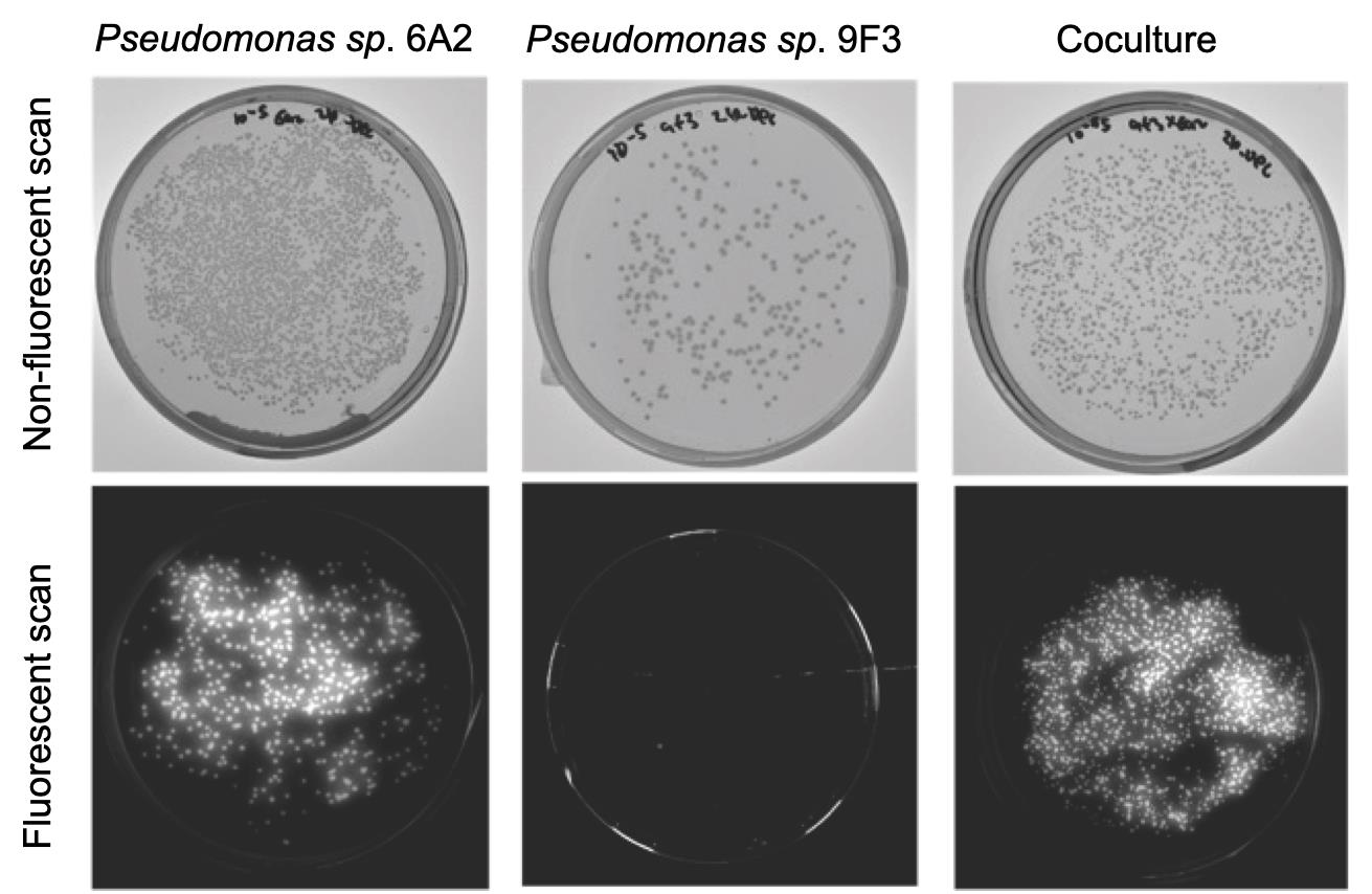
Figure 2. Distinguishing fluorescent Pseudomonas sp. 6A2 strains with a non-fluorescent Pseudomonas sp. 9F3 for colony-forming unit (CFU) counts in coculture. Fluorescent scan provides no CFUs for non-fluorescent strains (bottom-middle panel), allowing estimation of both fluorescent and non-fluorescent strains in coculture.
8. Count the number of colonies using ImageJ and use it for calculating interaction scores using the formula below:
Interaction score strainA = Log2 (CFU of strain A in coculture/CFU of strain A in monoculture)
Interaction score strainB = Log2 (CFU of strain B in coculture/CFU of strain B in monoculture)
Figure 3 shows a representative result of interaction scores from selected bacterial pairs from their in vitro culture.
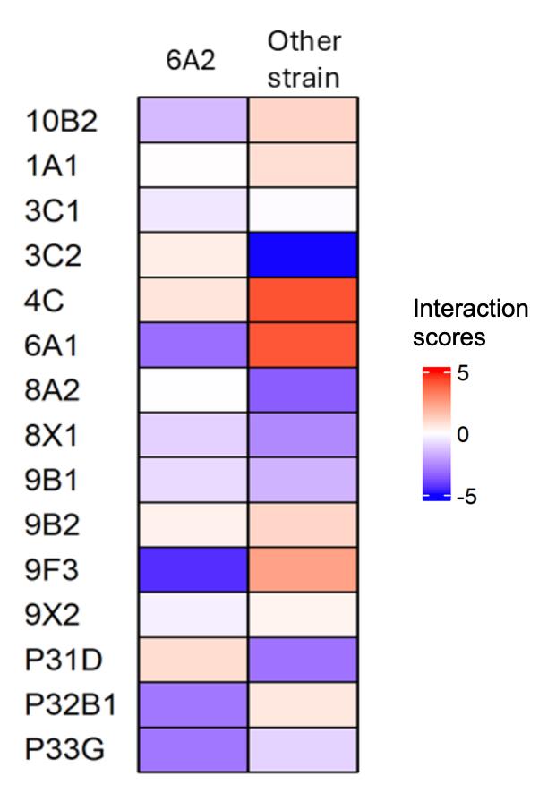
Figure 3. Interaction scores of Pseudomonas sp. 6A2 with 15 other strains from their in vitro culture. The first column indicates the interaction scores of 6A2 with other strains (in rows), and the second column indicates the interaction score of other strains in coculture with Pseudomonas sp. 6A2. This figure is created using the ComplexHeatmap package in R (v 4.4.1).
Based on the nature of their interactions (Figure 3), we summarized their ecological interactions obtained from their in vitro validation in Table 2 below. These interactions were varied, with at least one species experiencing negative effects in coculture for the majority of the pairs (Table 2).
Table 2. Nature of ecological interactions within a bacterial pair in vitro. The signs indicate negative (-), positive (+), or neutral (0) effects experienced in Strain 1 in the presence of Strain 2.
| Strain 1 | Strain 2 | Type of ecological interaction |
|---|---|---|
| 10B2 | 6A2 | Exploitative (-,+) |
| 1A1 | 6A2 | Amensal (0,-) |
| 3C1 | 6A2 | Neutral (0,0) |
| 3C2 | 6A2 | Amensal (0,-) |
| 4C | 6A2 | Commensal (0,+) |
| 6A1 | 6A2 | Exploitative (-,+) |
| 8A2 | 6A2 | Amensal (0,-) |
| 8X1 | 6A2 | Competitive (-,-) |
| 9B1 | 6A2 | Competitive (-,-) |
| 9B2 | 6A2 | Commensal ((0,+) |
| 9F3 | 6A2 | Competitive (-,-) |
| 9X2 | 6A2 | Neutral (0,0) |
| P31D | 6A2 | Exploitative (+,-) |
| P32B1 | 6A2 | Amensal (-,0) |
| P33G | 6A2 | Competitive (-,-) |
9. Calculate the correlation between the predicted and in vitro estimated interaction scores using correlation estimates. We obtained a moderate and significant correlation between the predicted and in vitro estimated interaction scores for 6A2 and other strains within the SynCom (Figure 4). Decide the correct estimate of correlation (Spearman for non-normal and Pearson for normal distribution) based on the underlying data distribution. The normality of data distribution can be checked with a Shapiro test (shapiro.test function in R).
Note: Each bacterial pair has two different interaction scores; therefore, there are twice as many data points for the number of interacting pairs.
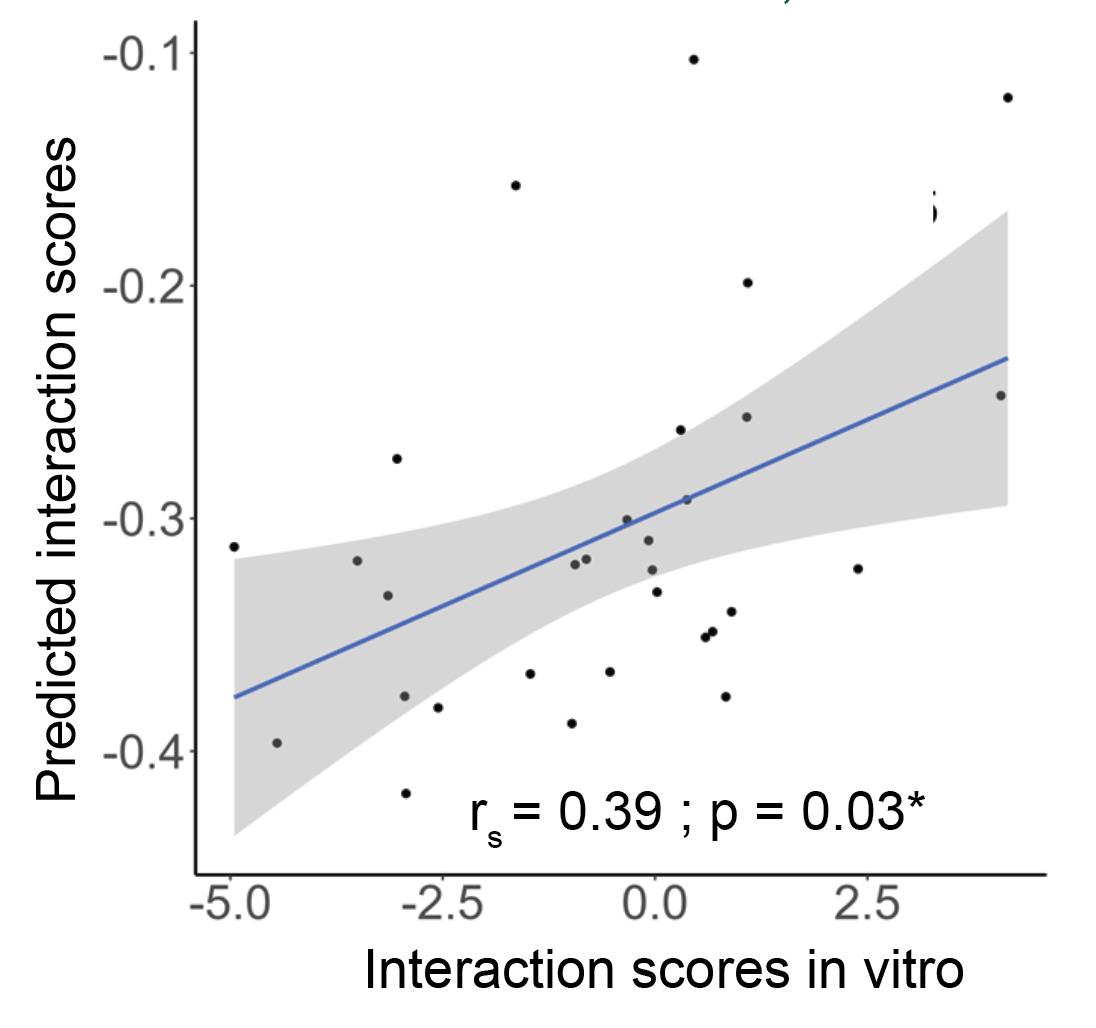
Figure 4. Correlation between predicted and in vitro validated interaction scores. The strength of correlation is calculated based on Spearman’s rank correlation, since the underlying data distribution is not normal. This figure is created using the ggplot2 package in R (v 4.4.1).
General notes and troubleshooting
General notes
1. For each bacterial pair, consider CFUs from at least three different dilutions for a more accurate representation.
2. Different metrics—growth rates and CFU counts—are used for in silico prediction and in vitro validation, respectively. Therefore, a moderate correlation strength between these two metrics (rs = 0.39) is expected, as found here. If two different bacterial strains are labeled with different fluorescent labels, growth rates can be estimated in their coculture. This is anticipated to provide better correlations. However, this is not feasible for a large number of strains.
3. The weak correlation between the predicted and in vitro validated interaction scores could be due to potential biological reasons. For example, metabolic models may not capture all signaling molecules, or the biomass objective function could be inaccurate.
Troubleshooting
Problem 1: No bacterial growth in ARE + MS medium.
Possible cause: pH of the media.
Solution: Check the pH of the media before filter sterilization. Ideally, the final ARE + MS mixed media should have a pH of 7.
Problem 2: No fluorescence of Pseudomonas strains.
Possible cause: Glycerol was not added to King’s agar B.
Solution: Ensure glycerol is added while preparing King’s agar B plates.
Problem 3: Installation of cplexsolver for running gapseq on Linux systems.
Possible cause: Incompatibility of cplexsolver.
Solution: Check the version compatibility of cplexsolver with your Linux specification.
Problem 4: Fluorescence bleeds between colonies.
Possible cause: Longer incubation time.
Solution: Before running the actual experiments, optimize the time of incubation to avoid overlap between colonies.
Problem 5: Weak correlation between the predicted and in vitro validated interaction scores.
Possible cause: GSMMs do not capture the complexity of signaling molecules or metabolites produced, or provide an incorrect biomass objective function.
Solution: Metabolic models could be curated further by testing for mass and charge balance, performing a leak test to ensure no metabolites could be produced from nothing, standardizing the metabolite namespace, adding reaction subsystems, and adding additional gene, metabolite, and reaction identifiers when available from reference genomes.
Problem 6: Poor quality score of metabolic models in MEMOTE.
Possible cause: Metabolic models are incomplete or do not follow the stoichiometry of the reactions.
Solution: Curate the metabolic models by considering similar approaches explained in Problem 5.
Data analysis
Growth rates of bacterial strains in monoculture and coculture were calculated using the growthcurver package in R. Average growth rates in coculture and monoculture were considered from three independent simulations. Similarly, CFU counts were considered as an average from three independent replicates of coculture and monoculture in a bacterial pair. The correlation coefficient between the in silico prediction and in vitro validation was calculated based on Spearman’s correlation, considering the non-normal distribution of data points. Estimation of the correlation coefficient in R (v 4.4.1) and the scatterplot was generated using the package ggplot2.
Calculation of growth rates:
The simulated growth files (.RDS extension) for each bacterium and their coculture with other bacteria were imported into R. The R package growthcurver was used to extract their growth rates and summarize them into a table. The detailed codes for this calculation can be found at https://github.com/arijitnus/Bio-protocol/blob/main/In%20silico%20prediction/growth_curve_params.R.
Calculation of interaction scores:
Interaction scores for each bacterial pair were estimated by taking the log2 of the ratio of growth rates in coculture to monoculture. For in vitro interactions, the interaction scores were calculated by taking the log2 of the ratio of CFUs in coculture to monoculture. The detailed codes for estimation of interaction scores can be found at https://github.com/arijitnus/Bio-protocol/blob/main/In%20silico%20prediction/Interactionscore_calc.R. The interactions were classified in ecological terms (e.g., commensal, amensal, competition) based on the signs (+/-) of interactions in a bacterial pair. For example, if two strains negatively impact each other’s growth, the interaction is deemed competitive.
Validation of protocol
The correlation (rs = 0.39) coefficient obtained as part of the in vitro validation is weak. There are two main reasons: (i) The metabolic models are incomplete, and (ii) different metrics are used for correlation. We propose that the improvement of metabolic models and the use of fluorescent strains to capture in vitro growth rates will improve the predictive accuracy. These strategies are further discussed in the General notes and Troubleshooting section. This protocol has been used and validated in the following research article:
Mukherjee et al. [16]. A bacterial signal coordinates plant-microbe fitness trade-off to enhance sulfur deficiency tolerance in plants. Cell Host Microbe. 2025 Sep 26: S1931-3128(25)00373-7. doi: 10.1016/j.chom.2025.09.007.
Supplementary information
The genome sequences are available in the public repository Zenodo, using the following identifier: https://zenodo.org/records/16929714. Quality metrics of the genomes can be found in Table S1.
The following supporting information can be downloaded here:
1. Table S1. Quality metrics of the SynCom genomes used in this protocol
2. File S1. SynCom sequences.zip
Acknowledgments
Conceptualization, A.M. and S.S.; Investigation, A.M. and B.H. Writing—Original draft, A.M.; Writing—Review & Editing, A.M.; Funding acquisition, S.S.; Supervision, S.S. Funding: Singapore Center for Environmental Life Sciences and Engineering. This protocol is used in the publication: Mukherjee et al. [16]. A bacterial signal coordinates plant-microbe fitness trade-off to enhance sulfur deficiency tolerance in plants. Cell Host Microbe. 2025 Sep 26: S1931-3128(25)00373-7. doi: 10.1016/j.chom.2025.09.007.
Competing interests
The authors declare no conflicts of interest.
References
- Turner, T. R., James, E. K. and Poole, P. S. (2013). The plant microbiome. Genome Biol. 14(6): 1–10. https://doi.org/10.1186/gb-2013-14-6-209
- Trivedi, P., Leach, J. E., Tringe, S. G., Sa, T. and Singh, B. K. (2020). Plant–microbiome interactions: from community assembly to plant health. Nat Rev Microbiol. 18(11): 607–621. https://doi.org/10.1038/s41579-020-0412-1
- Hassani, M. A., Durán, P. and Hacquard, S. (2018). Microbial interactions within the plant holobiont. In Microbiome (Vol. 6, Issue 1, p. 58). https://doi.org/10.1186/s40168-018-0445-0
- Maynard, D. S., Miller, Z. R. and Allesina, S. (2019). Predicting coexistence in experimental ecological communities. Nat Ecol Evol. 4(1): 91–100. https://doi.org/10.1038/s41559-019-1059-z
- Friedman, J., Higgins, L. M. and Gore, J. (2017). Community structure follows simple assembly rules in microbial microcosms. Nat Ecol Evol. 1(5). https://doi.org/10.1038/s41559-017-0109
- Schäfer, M., Pacheco, A. R., Könzler, R., Bortfeld-Miller, M., Field, C. M., Vayena, E., Hatzimanikatis, V. and Vorholt, J. A. (2023). Metabolic interaction models recapitulate leaf microbiota ecology. Science (1979). 381(6653): 42–55. https://doi.org/10.1126/science.adf5121
- Quinn-Bohmann, N., Carr, A. V., Diener, C. and Gibbons, S. M. (2025). Moving from genome-scale to community-scale metabolic models for the human gut microbiome. Nat Microbiol. 10(5): 1055–1066. https://doi.org/10.1038/s41564-025-01972-2
- Gu, C., Kim, G. B., Kim, W. J., Kim, H. U. and Lee, S. Y. (2019). Current status and applications of genome-scale metabolic models. Genome Biol. 20(1): e1186/s13059–019–1730–3. https://doi.org/10.1186/s13059-019-1730-3
- Salas-González, I., Reyt, G., Flis, P., Custódio, V., Gopaulchan, D., Bakhoum, N., Dew, T. P., Suresh, K., Franke, R. B., Dangl, J. L., et al. (2021). Coordination between microbiota and root endodermis supports plant mineral nutrient homeostasis. Science (1979). 371(6525): eabd0695. https://doi.org/10.1126/science.abd0695
- Helfrich, E. J. N., Vogel, C. M., Ueoka, R., Schäfer, M., Ryffel, F., Müller, D. B., Probst, S., Kreuzer, M., Piel, J. and Vorholt, J. A. (2018). Bipartite interactions, antibiotic production and biosynthetic potential of the Arabidopsis leaf microbiome. Nat Microbiol. 3(8): 909–919. https://doi.org/10.1038/s41564-018-0200-0
- Wang, N. R., Wiesmann, C. L., Melnyk, R. A., Hossain, S. S., Chi, M.-H., Martens, K., Craven, K., Haney, C. H. and Guttman, D. S. (2022). Commensal Pseudomonas fluorescens Strains Protect Arabidopsis from Closely Related Pseudomonas Pathogens in a Colonization-Dependent Manner. Retrieved from https://journals.asm.org/journal/mbio
- Getzke, F., Hassani, M. A., Crüsemann, M., Malisic, M., Zhang, P., Ishigaki, Y., Böhringer, N., Jiménez Fernández, A., Wang, L., Ordon, J., et al. (2023). Cofunctioning of bacterial exometabolites drives root microbiota establishment. Proc Natl Acad Sci USA. 120(15): e2221508120. https://doi.org/10.1073/pnas.2221508120
- Schneider, C. A., Rasband, W. S. and Eliceiri, K. W. (2012). NIH Image to ImageJ: 25 years of image analysis. Nat Methods. 9(7): 671–675. https://doi.org/10.1038/nmeth.2089
- Lieven, C., Beber, M. E., Olivier, B. G., Bergmann, F. T., Ataman, M., Babaei, P., Bartell, J. A., Blank, L. M., Chauhan, S., Correia, K., et al. (2020). MEMOTE for standardized genome-scale metabolic model testing. Nat Biotechnol. 38(3): 272–276. https://doi.org/10.1038/s41587-020-0446-y
- Zimmermann, J., Kaleta, C. and Waschina, S. (2021). Gapseq: Informed Prediction of Bacterial Metabolic Pathways and Reconstruction of Accurate Metabolic Models. Genome Biol. 22(1): 1–35. https://doi.org/10.1186/s13059-021-02295-1
- Mukherjee, A., Mazumder, M., Verma, A., Tikariha, H., Bhattacharya, R., Ooi, Q. E. and Swarup, S. (2025). A bacterial signal coordinates plant-microbe fitness trade-off to enhance sulfur deficiency tolerance in plants. Cell Host Microbe. 33(10):1748–1764.e6. https://doi.org/10.1016/j.chom.2025.09.007
Article Information
Publication history
Received: May 21, 2025
Accepted: Sep 25, 2025
Available online: Oct 15, 2025
Published: Nov 5, 2025
Copyright
© 2025 The Author(s); This is an open access article under the CC BY-NC license (https://creativecommons.org/licenses/by-nc/4.0/).
How to cite
Mukherjee, A., Tan, B. H. and Swarup, S. (2025). In Silico Prediction and In Vitro Validation of Bacterial Interactions in the Plant Rhizosphere Using a Synthetic Bacterial Community. Bio-protocol 15(21): e5496. DOI: 10.21769/BioProtoc.5496.
Category
Bioinformatics and Computational Biology
Microbiology > Microbe-host interactions > Bacterium
Plant Science > Plant immunity > Host-microbe interactions
Do you have any questions about this protocol?
Post your question to gather feedback from the community. We will also invite the authors of this article to respond.