- Protocols

- Articles and Issues
- For Authors
- About
- Become a Reviewer

Optogenetic Approach for Investigating Descending Control of Nociception in Ex Vivo Spinal Cord Preparation
Published: Vol 15, Iss 21, Nov 5, 2025 DOI: 10.21769/BioProtoc.5483 Views: 1976
Reviewed by: Anonymous reviewer(s)
Original research article
The authors used this protocol in:
Apr 2019

Protocol Collections
Comprehensive collections of detailed, peer-reviewed protocols focusing on specific topics


Related protocols
Abstract
Nociception is critically shaped by descending modulation of spinal circuits, yet its cellular and synaptic mechanisms remain poorly defined. Elucidating these mechanisms is technically challenging, as it requires simultaneous activation of primary afferents and descending fibers while monitoring the functioning of individual spinal neurons. Here, we present a method to investigate the influence of the rostral ventromedial medulla (RVM), a principal supraspinal structure mediating descending modulation, on the activity of spinal lamina I neurons. Our approach combines electrophysiological recordings in ex vivo intact spinal cord preparation with optogenetics, granting several advantages. First, ex vivo preparation spares rostrocaudal and mediolateral spinal architecture, preserving lamina I as well as primary afferent and descending inputs. Second, virally mediated channelrhodopsin-2 (ChR2) expression enables selective photostimulation of RVM-originating fibers. When coupled with patch-clamp recordings, this photostimulation allows identifying postsynaptic inputs from RVM to spinal neurons and revealing RVM-dependent presynaptic inhibition of primary afferent inputs. Overall, our approach is well-suited for investigating both pre- and postsynaptic mechanisms of descending modulation in physiological and pathological pain conditions.
Key features
• Rapid preparation procedure that grants access to lamina I neurons while preserving spinal cord architecture, including primary afferents and descending inputs.
• Optogenetic approach allowing functional studies of RVM-dependent descending modulation.
• Ability to assess RVM fiber–dependent presynaptic inhibition of synaptic transmission between primary afferents and lamina I neurons.
Keywords: OptogeneticsGraphical overview
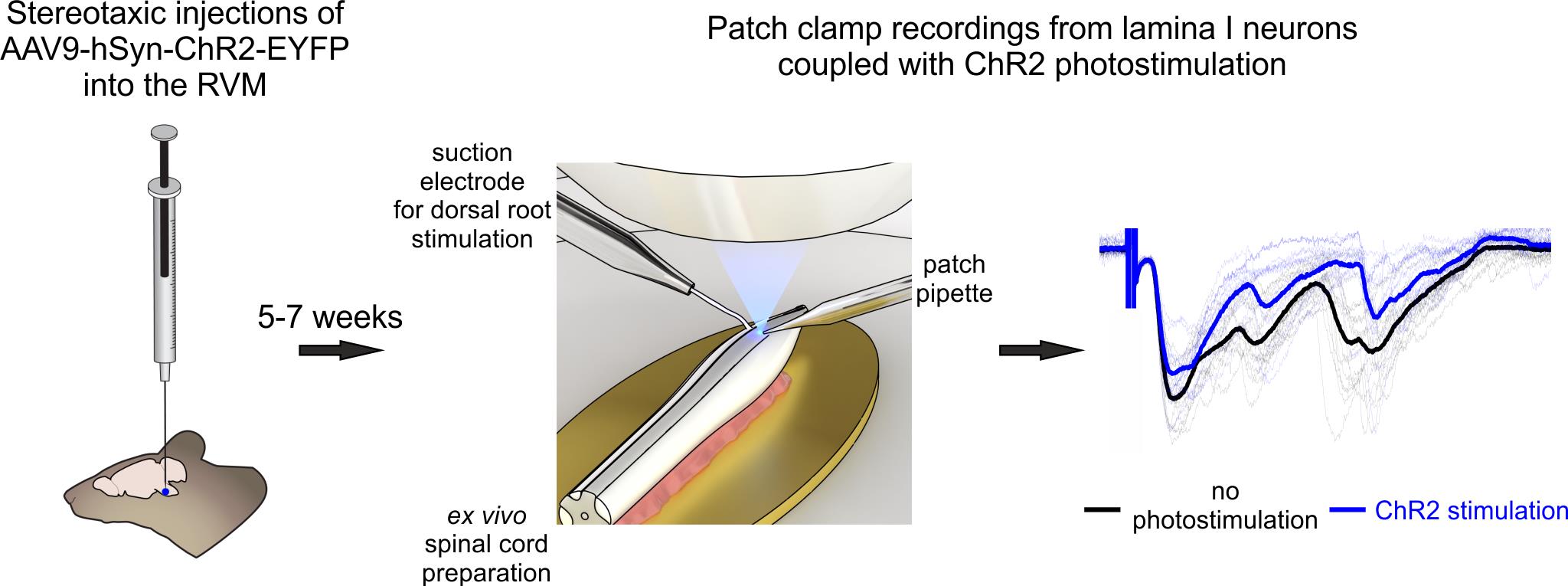
Optogenetic approach for functional studies of rostral ventromedial medulla (RVM)-dependent descending control of spinal lamina I neurons
Background
Neurons of the superficial dorsal horn (spinal laminae I–II) receive direct input from high-threshold primary afferents, perform primary processing of nociceptive signals, and relay pain-related information to the brain [1,2]. At the same time, this important ascending pathway is subject to descending feedback control. Several supraspinal structures located mostly in the hindbrain modulate the functioning of nociceptive-processing spinal neurons, thereby facilitating or inhibiting pain sensations [3–5]. Therefore, understanding the mechanisms of descending modulation is essential for advancing pain research.
Unfortunately, descending modulation remains poorly studied due to technical challenges that arise from the intrinsic organization of the central nervous system. Spinal and supraspinal structures are spatially separated (even in mice, they are a few centimeters apart), making it difficult to preserve both for functional studies. To address this challenge, several different approaches have been developed. The first one involves single-unit recordings from spinal neurons coupled with electrical stimulations of brainstem regions [6–8]. Although this method provides valuable information on how descending regulation affects action potential generation in spinal neurons, it offers no insight into its cellular and synaptic mechanisms. Besides, this method is difficult to apply to lamina I, as it is an extremely thin layer extending only about 30 μm from the surface of the dorsal horn. The second approach involves patch-clamp recordings in ex vivo spinal cord preparation combined with electrical stimulations of various descending spinal cord tracts [9]. While this technique is more suited for mechanistic studies, it cannot distinguish the impact of individual supraspinal structures, as their fibers largely travel within the same dorsolateral funiculus. Lastly, the third approach relies on optogenetics, i.e., virally mediated expression of light-sensitive channelrhodopsin-2 protein in the axons and terminals of descending fibers [10]. Combining patch-clamp recordings from superficial dorsal horn neurons with selective, photostimulation-induced activation of descending fibers originating from a single supraspinal source offers a unique possibility to determine how specific brain structures exert descending control. However, this method requires slicing the spinal cord, which damages lamina I and compromises primary afferent input—an important limitation, as descending fibers are known to modulate synaptic transmission between primary nociceptors and spinal neurons through presynaptic mechanisms.
Here, we provide a detailed protocol integrating patch-clamp recordings from lamina I neurons of intact ex vivo spinal cord preparation with optogenetic stimulation of descending fibers originating from rostral ventromedial medulla (RVM), a key hindbrain region mediating descending control. The main advantages of the proposed procedure are a) selective activation of RVM fibers, b) sparing the dendritic and axonal arborization of lamina I neurons, and c) preservation of the entire rostrocaudal and mediolateral spinal cord architecture, including all primary afferent input and RVM connections, important for studying both pre- and postsynaptic mechanisms of descending regulation. Compared to other methods that rely on slicing, ex vivo spinal cord preparation is faster and more reliable; the preparation is ready within 30–40 min after decapitation, it does not require any additional incubation, and may be used for up to 6–8 hours. Furthermore, cell visualization is performed using infrared LED oblique illumination [11,12], which does not require any sophisticated equipment for differential interference contrast.
Our protocol is well-suited for investigating RVM-dependent descending modulation under both physiological and pathological pain conditions. It can also be readily adapted to study descending control mediated by other supraspinal structures, such as the dorsal reticular nucleus and parabrachial nucleus. The electrophysiological recordings described here are compatible with pharmacological investigations and can be combined with Ca2+ transient measurements using either membrane-impermeable or genetically encoded Ca2+ indicators.
Since the protocol uses mice as the model organism, it is compatible with a wide range of transgenic lines, enabling flexible experimental design. In particular, animals expressing GFP in glutamatergic, GABAergic, or glycinergic neurons can help elucidate the mechanisms of descending modulation in distinct populations of spinal neurons. Lastly, retrograde labeling of lamina I projection neurons may offer valuable insights into how supraspinal structures influence the transmission of nociceptive signals to higher brain centers.
Materials and reagents
Biological materials
1. 12–15-week-old mice (any strain)
2. AAV9-hSyn-hChR2(H134R)-EYFP (titer ≥ 1 × 10¹³ vg/mL) (AddGene, catalog number: 26973-AAV9)
Reagents
1. Sucrose (Merck, catalog number: S0389)
2. Glucose (Merck, catalog number: G8270)
3. Sodium chloride (NaCl) (Merck, catalog number: S9888)
4. Sodium bicarbonate (NaHCO3) (Merck, catalog number: S0751)
5. Sodium monophosphate (NaH2PO4) (Merck, catalog number: S6040)
6. Potassium chloride (KCl) (Merck, catalog number: P9333)
7. Magnesium chloride (MgCl2·6H2O) (Merck, catalog number: M2670)
8. Calcium chloride (CaCl2·2H2O) (Merck, catalog number: C7902)
9. Potassium gluconate (Merck, catalog number: G4500)
10. Sodium ATP (Na2ATP) (Merck, catalog number: A3377)
11. Sodium GTP (NaGTP) (Merck, catalog number: G8877)
12. HEPES (Merck, catalog number: H3375)
13. EGTA (Merck, catalog number: E0396)
14. Sodium ascorbate (Merck, catalog number: 11140)
15. Sodium pyruvate (Merck, catalog number: P2256)
16. Potassium hydroxide (KOH) (Honeywell-Fluka, product number: 15653560)
17. Anesthetic agents: ketamine hydrochloride (50 mg/mL, Farmak) and sedazin (20 mg/mL, xylazine, Biowet Pulawi) or isoflurane (Abbvie, catalog number: B506)
18. Mineral oil (Merck, catalog number: M5904)
19. 95% O2 and 5% CO2 gas mixture (locally sourced)
20. O2 gas (in case isoflurane anesthesia is used for stereotaxic injections)
Solutions
1. Sucrose dissection solution (see Recipes)
2. Krebs bicarbonate solution (see Recipes)
3. Potassium gluconate intracellular solution (see Recipes)
Recipes
1. Sucrose dissection solution
| Reagent | Final concentration | Quantity |
|---|---|---|
| Sucrose | 200 mM | 34.23 g |
| Glucose | 11 mM | 991 mg |
| NaHCO3 | 26 mM | 1.092 g |
| NaH2PO4 | 1.2 mM | 72 mg |
| KCl | 2 mM | 74.5 mg |
| MgCl2·6H2O | 7 mM | 712 mg |
| CaCl2·2H2O | 0.5 mM | 37 mg |
| Sodium ascorbate (optional) | 5 mM | 495 mg |
| Sodium pyruvate (optional) | 3 mM | 168 mg |
| ddH2O | to 0.5 L |
pH is 7.3–7.4 when bubbled with 95% O2 and 5% CO2. Osmolarity is 310–320 mOsm/kg.
This solution may be used for up to 10 days after preparation if kept at 4–8 °C.
2. Krebs bicarbonate solution
| Reagent | Final concentration | Quantity |
|---|---|---|
| NaCl | 125 mM | 3.653 g |
| Glucose | 10 mM | 901 mg |
| NaHCO3 | 26 mM | 1.092 g |
| NaH2PO4 | 1.25 mM | 75 mg |
| KCl | 2.5 mM | 93 mg |
| MgCl2·6H2O | 1 mM | 102 mg |
| CaCl2·2H2O | 2 mM | 147 mg |
| ddH2O | to 0.5 L |
pH is 7.3–7.4 when bubbled with 95% O2 and 5% CO2. Osmolarity is 300–310 mOsm/kg.
This solution may be used for up to 10 days after preparation if kept at 4–8 °C.
3. Potassium gluconate intracellular solution
| Reagent | Final concentration | Quantity |
|---|---|---|
| Potassium gluconate | 145 mM | 1.698 g |
| MgCl2·6H2O | 2.5 mM | 25.5 mg |
| Sodium ATP | 2 mM | 55 mg |
| Sodium GTP | 0.5 mM | 13 mg |
| HEPES | 10 mM | 119 mg |
| EGTA | 0.5 mM | 9.5 mg |
| ddH2O | to 50 mL |
Adjust pH to 7.3 with 1 M KOH solution. Osmolarity is 280–290 mOsm/kg.
Make 1 mL aliquots and freeze them at -20 °C.
Laboratory supplies
1. Dissection dish with Sylgard-lined bottom (Living Systems Instrumentation, catalog number: DD-90-S-BLK)
2. 25 G hypodermic needles (BD, catalog number: 300400)
3. 30 G hypodermic needles (BD, catalog number: 304000)
4. Super glue (cyanoacrylate, water-resistant gel)
5. Glass capillaries with filament O.D. 1.5 mm, I.D. 0.86 mm (e.g., Sutter Instruments, catalog number: BF-150-86-10; Harvard Apparatus, catalog number: GC150F-10)
6. Thin-walled glass capillaries without filament O.D. 1.5 mm, I.D. 1.17 mm (Warner Instruments, catalog number: G150T-3)
7. 1 mL Luer-Lok syringes (BD, catalog number: 309628)
8. 2.5 mL Luer-Lok syringes (BD, catalog number: 300185)
9. Silicon tubing (VWR, catalog number: 228-0701)
10. Three-way tap (BD Connecta, catalog number: 394601)
11. MicroFil pipette fillers (WPI, catalog number: MF28G67-5)
12. Sterile syringe filters 0.22 μm (Thermo Scientific, catalog number: 171-0020)
13. Glass capillaries for stereotaxic syringe (Sutter instruments, catalog number: BF100-50-10)
14. Surgical sutures or staples
15. Disposable laboratory gloves (any suitable ones)
16. Parafilm (Merck, catalog number: HS234526B)
17. Eye ointment (Vidisic, Bausch+Lomb)
18. 70% ethanol
19. Antiseptic solution (Betadine, 100 mg/mL, EGIS)
20. 1 mL insulin 29 G fixed needle syringes (BD Micro-Fine, catalog number: 324891)
21. Acrylic adhesive/dental cement (Stoelting, catalog number: 51459)
Equipment
Stereotaxic injections
1. Stereotaxic apparatus (David Kopf Instruments, model: 902 dual)
2. Syringe for stereotaxic injections (10 μL, 701 Hamilton syringe with removable needle, catalog number: 80314)
3. 1 mm Hamilton micropipette compression fitting set (Hamilton, catalog number: 55750-01RN)
4. Manual injector/micrometer (Starrett, model: 262M) or an automatic injection pump
5. Rodent warming system (Stoelting, model: 53800 series)
6. Fur clipper (Kent Scientific, model: CL7300-KIT)
7. Bead sterilizer (Merck, catalog number: Z378569)
8. Microdrill (Stoelting, product number: 58610V) and respective drill bits (preferably 0.6 mm, Stoelting, catalog number: 58609)
9. Optional: Rodent anesthesia system (VetEquip)
Dissection instruments
1. Dissection pad (could be made from Styrofoam tightly wrapped in foil)
2. Big scissors (F.S.T., catalog number: 14000-20)
3. Small scissors (F.S.T., catalog number: 14058-11)
4. Coarse forceps (F.S.T., catalog number: 11651-10)
5. Big spring scissors (F.S.T., catalog number: 15025-10)
6. Small spring scissors (F.S.T., catalog number: 15000-12)
7. Two curved forceps (F.S.T., catalog number: 11063-07)
8. Fine forceps (F.S.T., catalog number: 11413-11)
9. Scalpel blade #15 (F.S.T., catalog number: 10015-00) and appropriate scalpel handle (F.S.T., catalog number: 10003-12)
10. Small metal plate (preferably gold, D.IY., ~1.5 cm × 1 cm, should fit in experimental chamber)
Visualization and illumination
1. Stereomicroscope (Olympus, model: SZX7)
2. Light source (AmScope, model: 6 W LED Dual Gooseneck Illuminator)
3. Upright microscope (Olympus, model: BX50WI)
4. 60× water immersion objective (Olympus, model: LUMPlanFl 60×/0.90 W)
5. Low magnification (4–5×) objective (Carl Zeiss, model: Epiplan; Olympus, model Plan N)
6. Eyepiece micrometer (Evident, model: U-OCMC10/100X)
7. Infrared-sensitive CCD camera (Olympus, model: OLY-150IR or Dage-MTI, model: IR-2000)
8. Narrow beam (± 3°) infrared light emitting diode (IR-LED, Osram, models: SFH4550, SFH4545)
Critical: The spectral characteristics of the IR-LED and CCD camera should match.
9. White light–emitting diode (Dialight, model: 5219901802F)
10. Power supply unit (AimTTI, model: QL355T)
11. Monochromator (Till Photonics, model: Polychrome V)
Note: Blue LED laser (wavelength ~470 nm) may also be used for photostimulation.
12. Filter set (any suitable for ChR2 and EYFP excitation, e.g., Chroma Technology, model: 69008)
Perfusion
1. Gravity-fed perfusion system (any commercially available or self-made)
2. Peristaltic pump (Gilson, model: Minipuls 3)
3. Recording chamber (any that fits the microscope)
Electrophysiology
1. Patch clamp amplifier with respective headstage (Molecular Devices, model: Multiclamp 700B, headstage CV-7B)
2. Digitizer (Molecular Devices, model: Digidata 1440)
3. PC computer with Windows operating system
4. Patch clamp micromanipulator (Scientifica, model: PatchStar)
5. Constant current stimulator (A.M.P.I., model: ISO-FLEX)
6. Vibration isolation table (CleanBench, model: TMC)
7. Faraday cage (any commercially available or self-made)
8. Small three-axis micromanipulators (Narishige, model: UN-3C)
9. Pipette holders (Molecular devices, model: 1-HL-U)
10. Pipette puller (Sutter Instruments, model: P-97)
11. Silver wire AWG 26 for electrodes (WPI, product number: AGW1510)
12. Ag/AgCl pellets (WPI, product number: EP1)
13. BNC cables
14. Bunsen burner
Software and datasets
1. pClamp (version 10.7, Molecular Devices, July 2016)
2. Clampfit (version 10.7, Molecular Devices, July 2016)
3. TillVision (version 4.0, Till Photonics, 2008) or alternative laser controlling software
4. Origin (version 2022, OriginLab, June 2022)
5. MiniAnalysis (version 6.0.37, Synaptosoft Inc., 2009)
Procedure
A. Stereotaxic injection
1. Autoclave necessary instruments (scalpel handle, spring scissors, curved forceps, etc.). Then, place them near the stereotaxic apparatus along with surgical sutures (staples).
2. Using a pipette puller and 1 mm capillaries, fabricate microinjection pipettes with a tip diameter between 10 and 50 μm and a taper length of 8–10 mm from the start of the taper.
Note: For detailed instructions on micropipette fabrication, refer to Chapter 10 of the Sutter Pipette Cookbook.
3. Slowly thaw a vial of AAV9-hSyn-hChR2(H134R)-EYFP viral construct.
Note: Keep the viral solution cooled at 4–8 °C throughout the procedure.
4. Prepare the syringe for injections.
a. Fill the barrel of a Hamilton (10 μL) syringe and the micropipette with mineral oil.
b. Insert the micropipette into the 1 mm Hamilton micropipette compression fitting set and securely connect it to the syringe (Figure 1A). Make sure there are no air bubbles in the micropipette.
c. Attach the syringe to the manual injector or automatic injection pump and mount the assembly onto the right arm (this configuration is more convenient for right-handed individuals) of the stereotaxic apparatus.
5. Anesthetize a mouse using the preferred anesthetic agent.
a. Ketamine/xylazine anesthesia:
i. In a vial, prepare a mixture of ketamine and xylazine solutions according to the animal’s weight (ketamine: 100 mg/kg; xylazine: 12 mg/kg).
ii. Transfer the anesthetic mixture to an insulin syringe with an integrated 29 G or 30 G needle.
iii. Administer the injection intraperitoneally and put the animal into an anesthesia induction chamber.
iv. Induction of anesthesia should occur within 3–4 min.
b. Isoflurane anesthesia:
i. Transfer the animal into an anesthesia induction chamber.
ii. Open the oxygen tank, set the pressure to 700 mmHg, and set the isoflurane concentration to 4%.
iii. Induction of anesthesia should occur within 1–2 min.
6. Remove the animal from the anesthesia induction chamber. Confirm the absence of a pedal withdrawal reflex by gently pinching the hind paw.
7. Mount the animal onto the stereotaxic apparatus (Figure 1B).
a. Position the snout in the central clamp of the stereotaxic apparatus, ensuring the upper front teeth fit securely into the groove at the base of the clamp. Gently tighten to secure the snout.
b. Insert one ear bar into the ear canal until it contacts the skull, aligning the skull with the snout clamp. Tighten the bar to hold it in place. Repeat on the opposite side, applying equal pressure to stabilize the head. Ensure both ear bars are positioned symmetrically by confirming an equal distance from the center.
Optional: In case of isoflurane anesthesia, set the isoflurane concentration to 2%–2.5% after securing the mouse onto the stereotaxic apparatus.
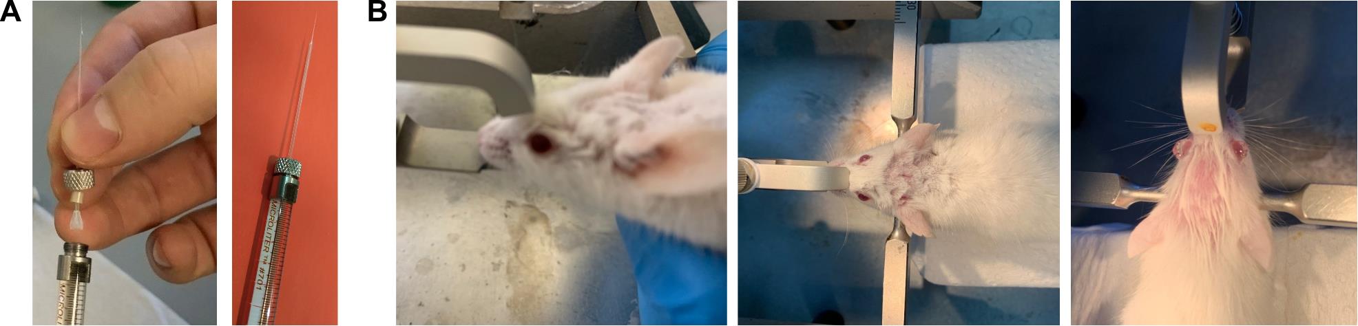
Figure 1. Stereotaxic injections. (A) Photographs showing the injection pipette and syringe used for the procedure. Left: connection of the microinjection pipette to the syringe. Right: fully assembled syringe with the attached microinjection pipette. The microinjection pipette should have a tip diameter between 10 and 50 μm and a taper length of 8–10 mm from the start of the taper. (B) Photographs demonstrating proper head positioning of the animal within the stereotaxic apparatus. Left: side view. Middle and right: top view.
8. Set the heating pad to 37 °C and position it beneath the animal to maintain body temperature.
9. Trim the fur on the mouse’s head. Then, apply an antiseptic solution (Betadine).
10. Apply a generous amount of topical eye ointment.
11. Using a scalpel, make a midline rostrocaudal incision extending from just behind the eyes to the occiput. Gently retract the skin to expose both the lambda and bregma points (Figure 2).
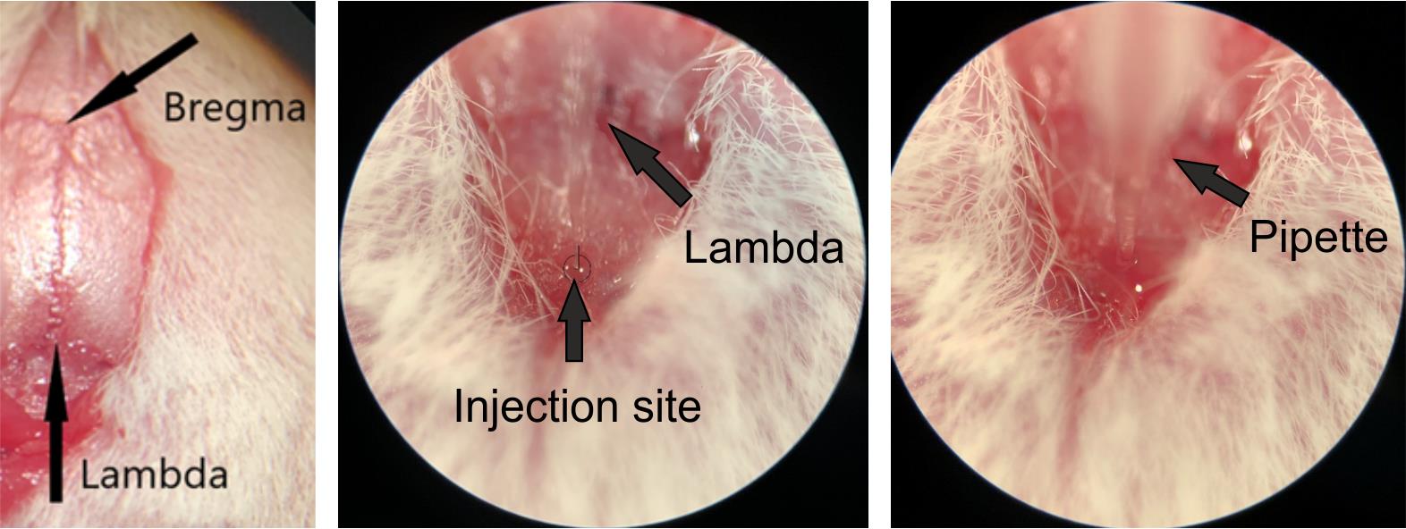
Figure 2. Determining the injection site. Photographs illustrating the injection site relative to the bregma and lambda points. Left: bregma and lambda points. Middle: injection site relative to the lambda point. Right: microinjection pipette inserted at the injection site. Note that the target location for rostral ventromedial medulla (RVM) injections is located directly on the suture of the midline, caudal to the lambda point, at a distance of 5.8 mm from the bregma.
12. Level the skull to ensure accurate stereotaxic targeting.
a. Attach a 30 G needle to the left arm of the stereotaxic frame.
b. Align the needle tip with the bregma and gently touch the skull surface to record the Z-axis coordinate.
c. Repeat this procedure for the following three reference points:
i. 2 mm lateral to the left of bregma.
ii. 2 mm lateral to the right of bregma.
iii. The lambda point.
d. Ensure that all Z-axis values match the bregma coordinate. If not, adjust the skull position to achieve a level orientation.
13. Once the skull is leveled, realign the needle with the bregma. Move it 5.8 mm caudally along the midline and gently press the tip into the midline suture of the skull to mark the drilling site (Figure 2).
Note: The drilling site is located directly on the suture of the midline.
14. Drill the skull using a microdrill. We recommend using the smallest drill bit (0.6 mm).
Note: In case a microdrill is not available, use a 29 G needle. Place the tip of the needle on the mark and apply light pressure while spinning the needle in your fingers until resistance from the skull disappears.
15. Place a piece of parafilm on the skull and position the microinjection pipette directly above it. Using a calibrated measuring pipette, dispense 50–100 nL of the viral solution onto the center of the Parafilm. Immediately lower the microinjection pipette into the droplet and gently retract the syringe plunger to aspirate the entire volume into the microinjection pipette. Then, lift the pipette and remove the parafilm.
16. Align the tip of the microinjection pipette with the center of the drilled hole and lower it until it reaches the opening. Then, slowly advance the pipette ventrally by 5.8 mm from the surface of the skull over the course of 1 min to reach the RVM. Once at the target depth, retract the pipette by 0.1–0.2 mm to reduce tissue pressure at the injection site.
17. Inject the viral construct at a rate of 1 nL/s. Upon completion of the injection, leave the micropipette in place for 5–10 min to allow for diffusion and minimize backflow. Then, slowly retract the pipette over the course of approximately 1 min.
18. Seal the drilled hole with a small amount of acrylic adhesive (dental cement).
19. Suture or staple the incision.
Optional: If the mice are not housed individually, apply additional tissue adhesive to reinforce the closure and prevent wound disruption.
20. Remove the mouse from the stereotaxic frame.
21. Keep the animal on the heating pad until it recovers from anesthesia. Then, transfer it to a cage.
B. Spinal cord preparation
Important: Allow at least 5 weeks after stereotaxic injection to ensure robust expression of channelrhodopsin-2.
Critical: Ensure that sucrose dissection solution is at room temperature (20–23 °C) and has been bubbled with a 95% O2/5% CO2 gas mixture for at least 15 min prior to starting the preparation.
1. Arrange the dissection instruments near the stereomicroscope and switch on the illumination.
2. Place the animal in an induction chamber and administer isoflurane to induce deep anesthesia. Confirm the absence of a pedal withdrawal reflex by gently pinching the hind paw. Once a surgical level of anesthesia is verified, perform rapid decapitation using large scissors. Allow the blood to drain for approximately 10 s prior to tissue collection.
3. Position the decapitated animal on the dissection pad and gently secure its limbs using 25 G needles, as illustrated in Figure 3.
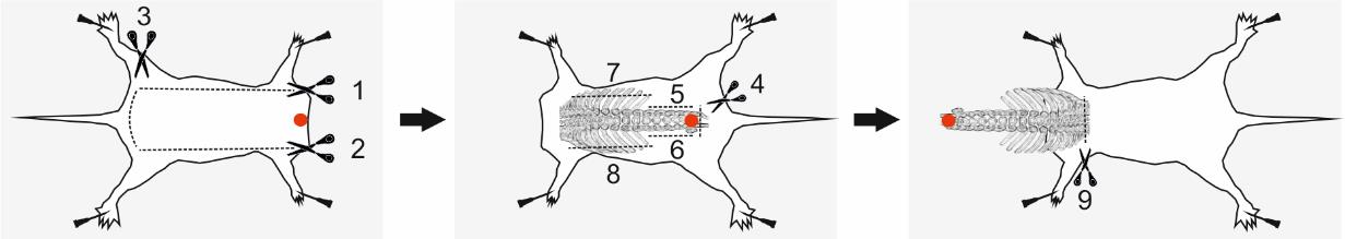
Figure 3. Spinal column excision. Schematic illustration of the excision process. Red dots indicate points to grasp with forceps; dashed lines represent the incision paths. Numbers denote the recommended sequence of cuts for a right-handed individual. Figure adapted from [13].
4. Remove the spinal column together with the attached ribs.
a. Carefully remove the skin from the back to expose the spinal column and ribs. Using coarse forceps, lift the skin and insert one blade of fine scissors underneath. While keeping the scissors parallel to the dissection pad, make an incision along one flank. Repeat the procedure along the opposite flank. Finally, cut the skin near the tail (Figure 3).
b. Hold the scissors vertically with the blades open and facing downward. Insert the scissors approximately 3–5 mm into the back at the level of the hips, positioning the blades on either side of the spinal column. Carefully sever the spinal column.
c. Using coarse forceps, grasp the cut end of the spinal column and gently lift it. With scissors, continue cutting the surrounding tissue rostrally along both sides of the column until you reach the ribs.
d. Cut the ribs on both sides and cut any thoracic or abdominal viscera that remain attached to the spinal column or rib cage.
Note: The ribs are essential for securing the preparation to the dissection dish. Avoid trimming them too short to ensure proper pinning.
e. With the spinal column held vertically, section it at the lower cervical or upper thoracic level.
5. Transfer the excised spinal column to a Sylgard-lined dissection dish containing sucrose solution aerated with 95% O2 and 5% CO2 gas mixture.
6. Using 30 G needles, secure the excised tissue with the dorsal side facing downward (ventral side upward), oriented rostrally toward the experimenter, as shown in Figure 4.
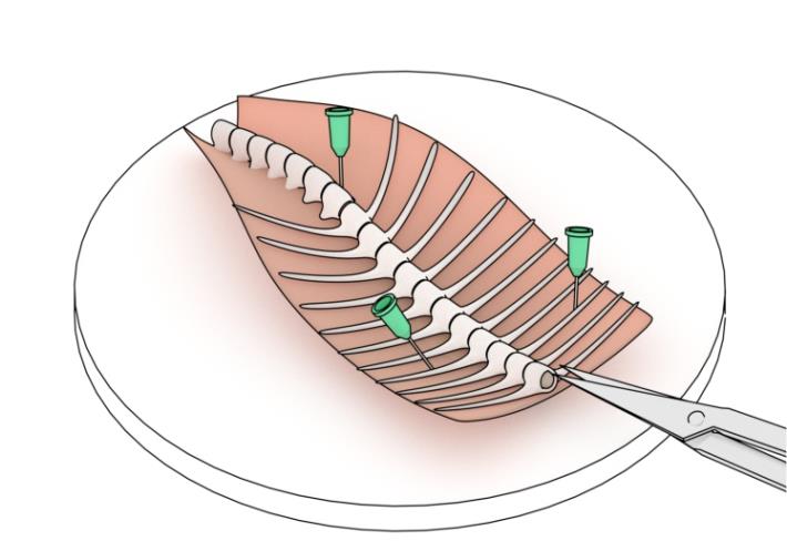
Figure 4. Schematic of pinning the preparation to the dissection dish. Note that three needles are used to secure the preparation to the bottom of the Sylgard-lined dissection dish. Note that the preparation is pinned at a 20–30○ angle relative to the experimenter’s line of sight (configuration suited for a right-handed individual). Figure adapted from [13].
7. Adjust the stereomicroscope to focus on the preparation using 8–10× magnification.
8. Using coarse forceps, grasp the ribs near the rostral end of the spinal column and gently lift to expose the opening. Insert one blade of the big spring scissors into the opening, pressing it against the vertebrae, and make a cut. Keeping the blades closed, angle the scissors to the side to withdraw them. Repeat the process on the opposite side of the vertebrae (Figure 5).
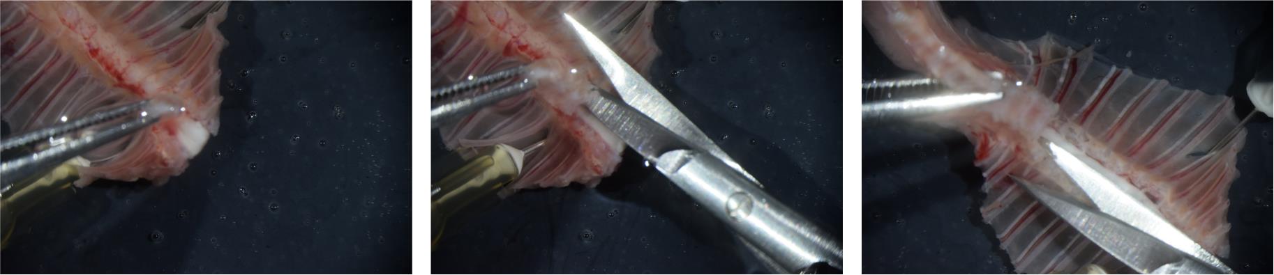
Figure 5. Removing the ventral portion of the vertebrae. Photographs illustrating the removal of the ventral portion of the vertebrae over lower cervical (left), upper thoracic (middle), and lower thoracic (right) spinal segments.
9. Using coarse forceps, grasp the cut ventral portion of the spinal column and gently pull it upward and caudally. This exposes the space between the spinal cord and vertebrae, where the scissor blade should be inserted. Continue cutting the vertebrae as previously described, keeping the scissors parallel to the dissecting dish (see Figure 5). Adjust the position of the forceps as you proceed, and exercise increased caution upon reaching the lumbar enlargement. Carefully cut any dura mater (an opaque sheath covering the spinal cord) attached to the ventral portion of the spinal column. Once the cauda equina (group of nerves and nerve roots stemming from the distal end of the spinal cord) is exposed (Figure 6), cut off the ventral part of the spinal column and remove it from the dish.
Optional: Cut the spinal meninges along the midline using small spring scissors.
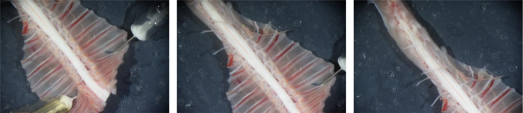
Figure 6. Exposed spinal cord. Photographs showing the exposed spinal cord. Note the removal of the ventral portion of the vertebrae and the exposure of the cauda equina. Left: lower cervical, thoracic, and lumbar spinal segments. Middle: thoracic, lumbar, and sacral spinal segments. Right: lumbar, sacral, and caudal segments.
10. Remove the spinal cord from the spinal column.
a. Cut the cauda equina.
b. Using the lateral surfaces of the vertebrae as a guide, cut the thoracic dorsal and ventral roots on both sides of the spinal cord.
c. With curved forceps, gently lift the spinal cord upward and to the side, then cut the dura mater connected to the dorsal aspect of the vertebrae. Ideally, hold the spinal cord by its rostral end, or preferably by the dura mater or thoracic roots (Figure 7).
Critical: Always keep the spinal cord submerged in aqueous solution. Avoid stretching the tissue at all times.
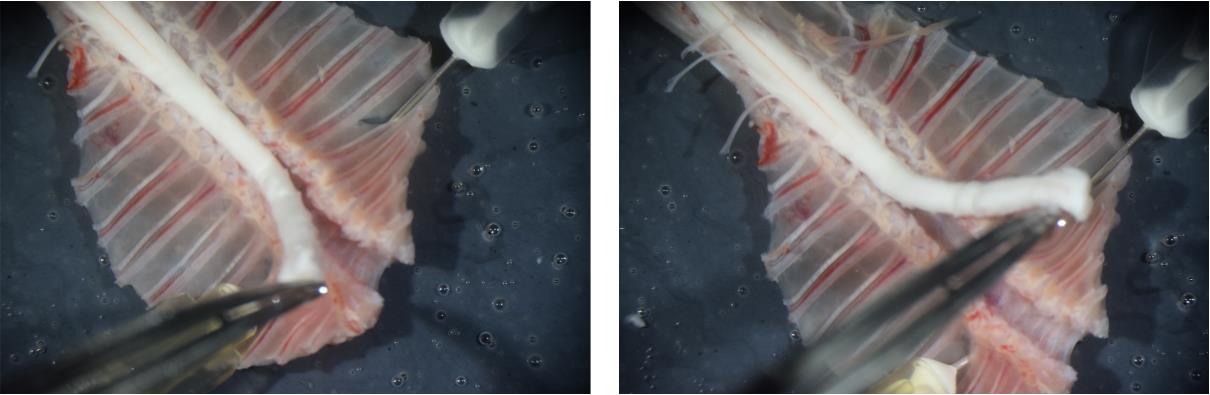
Figure 7. Removing the spinal cord from the spinal column. Photographs illustrating spinal cord handling during the removal process. Note that the spinal cord is held by its rostral end.
d. Sever the lumbar dorsal roots while preserving their full length.
e. Remove any remaining tissue anchoring the spinal cord to the interior of the vertebral column.
f. Fully remove the spinal cord and discard the spinal column with attached ribs.
Note: All the above steps should be completed within 7–10 min after decapitation. Longer preparation time decreases the number of neurons that are fit for recordings.
11. Position the spinal cord with the ventral side facing down. Carefully cut the spinal meninges along the midline using small spring scissors. Trim the most rostral portion of the spinal cord if it is extensively damaged. Then, pin the preparation to the dissecting dish with 30 G needles at the rostral and caudal ends (Figure 8).
12. Using curved or fine forceps, carefully remove the remaining dura mater covering the dorsal surface of the spinal cord and dorsal roots (Figure 8). Begin at the rostral end and gently peel the dura mater caudally until it is fully removed along the entire length of the spinal cord. Take care not to damage the lower lumbar dorsal roots. If necessary, use small spring scissors to make small incisions around the dorsal roots and remove the dura mater in separate pieces. By the end of this step, the individual dorsal roots should be clearly separated.
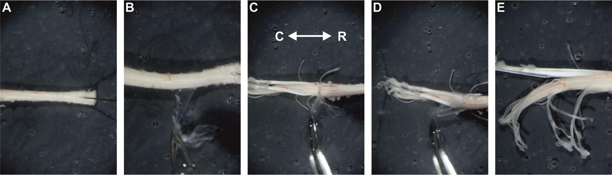
Figure 8. Removing the dura mater. Photographs illustrating different stages of dura mater removal. Care should be taken to avoid severing the lower lumbar dorsal roots. (A) Rostral end of the preparation pinned to the dissection dish with a 30G needle. (B–D) Removal of the dura mater over thoracic (B) and lumbar (C, D) spinal segments. (E) Lumbar spinal segment and dorsal roots after dura mater removal. R: rostral; C: caudal.
13. Remove the spinal meninges, including arachnoid and pia mater, from the side intended for experimentation.
a. Using fine forceps, pinch the rostral part of the spinal cord and pull the meninges.
b. Carefully peel the meninges caudally until the upper lumbar segments are reached (Figure 9).
Notes:
1. The pia mater contains prominent blood vessels; successful removal of the pia is indicated by the detachment of these vessels.
2. Peeling off the pia mater typically detaches dorsal and ventral roots in the thoracic segment.
c. Critical: Use small spring scissors to incise the meninges along the border between the dorsal horn and dorsal white matter. This step is necessary to spare the desired dorsal roots.
d. Continue peeling the meninges that span underneath the dorsal roots and cover the dorsal horn.
Important: For successful electrophysiological experiments, the meninges covering the dorsal horn underneath L4 and L5 dorsal roots should be fully removed. DO NOT remove the meninges above the dorsal white matter to avoid severing the desired dorsal roots.
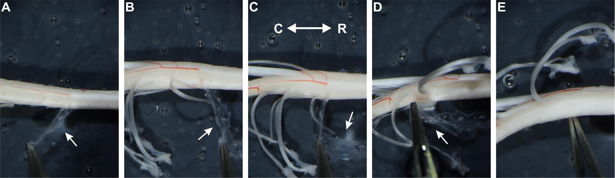
Figure 9. Removing the meninges. Photographs illustrating different stages of meninge removal. Note that removal of the pia mater is indicated by the detachment of the blood vessels. (A–C) Meninges removal over thoracic (A) and upper lumbar (B, C) spinal segments. (D) Meninges removal under L4 dorsal root. (E) Lower lumbar segments after meninge removal. Meninges covering the dorsal horn underneath L4 and L5 dorsal roots are fully removed. White arrows show the meninges. R: rostral; C: caudal.
14. Spare L4 and L5 dorsal roots and cut any remaining dorsal and ventral roots that are not intended for experiments. Position the preparation as shown in Figure 10.
Note: To identify L4–5 dorsal roots, first locate the L3 dorsal root, which covers the widest part of the lumbar enlargement. The L4 dorsal root lies caudally adjacent to L3, while the L5 dorsal root lies caudally adjacent to L4 on the conical part of the lumbar enlargement. We recommend preserving two dorsal roots, even if only one is intended for use in the experiments. This provides a backup in case one root becomes contaminated with glue during the mounting process.
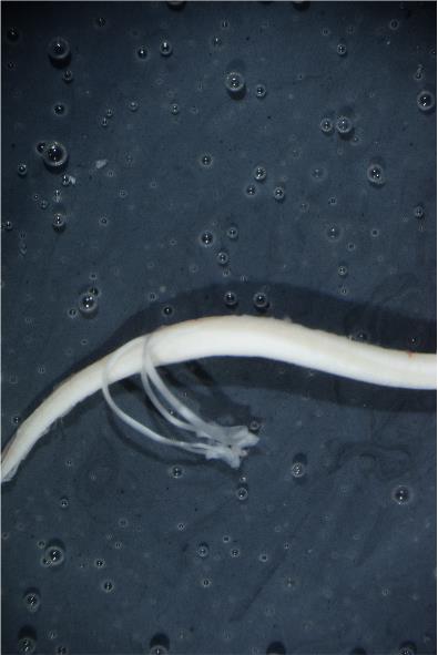
Figure 10. Spinal cord with spared L4 and L5 roots and removed meninges. Position the spinal cord in such a manner before proceeding to step B15. Notice spared L4 and L5 dorsal roots.
15. Glue the preparation to the metal plate.
a. Position the metal plate on the base of the stereomicroscope, near the dissection dish.
b. Use a 30 G needle to spread the cyanoacrylate glue, forming a thin, even layer over half of the metal plate. Leave some glue on the tip of the needle for further use.
c. Using two curved forceps, hold the spinal cord at its rostral and caudal ends. Carefully lift the preparation from the aqueous solution and gently place it onto the section of the metal plate that is not coated with glue.
d. Slightly stretch the preparation, slightly lift above the metal plate, and put the spinal cord on the glue-covered part of the plate. Avoid gluing the dorsal roots.
Critical: Position the spinal cord at approximately 45○ angle, so that the dorsal horn is on the top (Figure 11). This orientation maximizes the number of cells visible under oblique illumination. Placing the spinal cord too flat or on its side substantially hinders further electrophysiological experiments.
e. Using a 30 G needle, apply more glue to the ventral side of the lumbar segment.
f. Transfer the metal plate with the glued spinal cord back to the aqueous solution.
Critical: Steps B15c–f should be performed within 20–30 s. Prolonged exposure to air damages the neurons within the superficial dorsal horn.
g. Optional: If one or both roots are exposed to the glue, gently detach them using a 30 G needle. Dorsal roots should float freely.
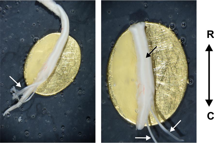
Figure 11. Ex vivo spinal cord preparation glued to a metal plate. Left: Spinal cord after mounting on the metal plate. Note that the dorsal roots are not glued and float freely. Right: Ex vivo spinal cord fully prepared and ready for experimentation. Note that the spinal cord is glued at approximately 45°, so that the dorsal horn is on the very top of the preparation. R: rostral; C: caudal. White arrows show the dorsal roots. The black arrow shows the dorsal horn.
16. Trim the rostral and caudal ends of the spinal cord that extend beyond the metal plate and are not securely adhered. Sever the dorsal roots that are not intended for experimentation; slightly pull the root with a forceps and cut as close to the spinal cord as possible.
Important: While using two dorsal roots for experiments can yield more data from each neuron, preserving only one root is often more practical, as it provides easier access to the rostrally adjacent spinal segment.
17. Remove dorsal root ganglia if they are attached to the roots. Cut dorsal roots to the desired length; use sharp scissors to avoid crushing the roots.
Note: Try to preserve the full extent of the dorsal roots. This would facilitate the distinction between A- and C-fiber-mediated components of primary afferent input.
Pause point: At this point, the preparation may be left in the oxygenated sucrose solution.
C. Setting up the perfusion system and transferring the preparation to the recording rig
1. Install the experimental chamber and position the patch clamp reference electrode.
2. Fill the perfusion system with Krebs bicarbonate solution. If the solution is recycled, ensure a minimum volume of 30–40 mL.
Note: Attach drippers to the outflow to minimize electrical noise from the peristaltic pump.
3. Set the perfusion flow rate to 1.5–3 mL/min. This can be achieved by using glass capillaries for both inflow and outflow; fire-polish their tips to obtain the desired diameter. Alternatively, a flow regulator may be used.
4. Verify that the flow through the chamber is stable and continuous—ripples in the bath should be avoided, as they can compromise patch-clamp stability.
5. Prior to transferring the preparation, bubble the Krebs solution thoroughly with a 95% O2/5% CO2 gas mixture for at least 5 min.
Critical: Krebs solution should be continuously bubbled throughout the whole experiment.
6. Bring the dissection dish with the preparation close to the recording chamber. Using forceps, gently grasp the metal plate to which the preparation is glued and transfer it into the chamber.
Important: Ensure the entire preparation, including the dorsal roots, remains fully submerged in solution at all times.
7. Align the metal plate so that the rostrocaudal axis of the preparation is parallel to either the x- or y-axis of the microscope stage.
8. Optional: At this stage, we recommend visualizing lamina I cells to confirm that the spinal cord is securely adhered to the metal plate. The image should be stable; no apparent vibration or wobbling should be observed. If any movement is detected, remove the preparation from the solution, gently dry the ventral side of the spinal cord with a Kimwipe, and reapply glue as needed.
D. Attaching dorsal roots to suction electrodes
Note: In the following steps, use a low-magnification objective (4×–5×) and a white LED for visualization.
1. Focus on the tip of the dorsal root and assess its width with either an eyepiece micrometer or camera software.
2 Fire-polish a thin-walled glass capillary to produce a suction electrode of the desired diameter. Use the microscope to examine the suction electrode; its opening should be slightly narrower than the width of the dorsal root.
Note: We advise fabricating a set of suction electrodes with various opening sizes (250–400 μm) beforehand and choosing an appropriate one during the experiment [13,14].
3. Insert the suction electrode into a pipette holder mounted on a manipulator. Connect the electrode to the anode of the constant current stimulator and attach the pipette holder to a 5 mL syringe using silicone tubing.
Note: We recommend using a compact manipulator with a magnetic base.
4. Lower the suction electrode into the recording chamber. Using the syringe, draw the bath solution into the electrode until it contacts the internal AgCl wire.
5. Bring the suction electrode opening close to the tip of the dorsal root (Figure 12). Align the electrode and the root as precisely as possible. If necessary, use forceps to gently adjust the root position. Apply negative pressure to draw the root into the electrode.
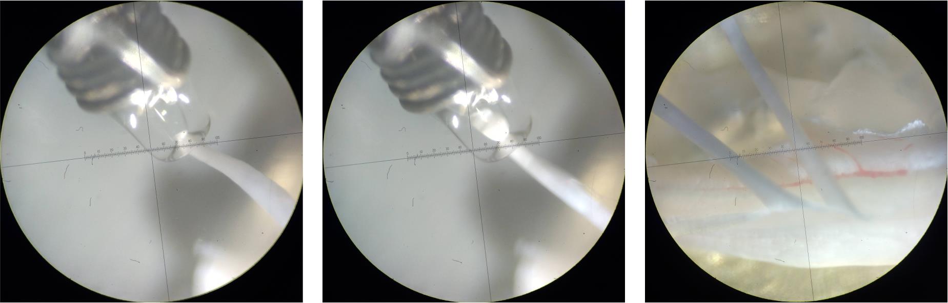
Figure 12. Attaching the dorsal root to the suction electrode. Photographs showing key stages of attaching the dorsal root to a suction electrode. Left: Before applying negative pressure, ensure the suction electrode and dorsal root are properly aligned. Note that the AgCl wire of the reference electrode is wrapped around the suction electrode. Middle: Dorsal root successfully attached. Observe the tight seal between the electrode and the root—only the distal tip of the root should enter the electrode. Right: Ex vivo spinal cord preparation ready for electrophysiological recordings. The suction electrodes apply slight tension to the dorsal roots, exposing the underlying dorsal horn.
6. Visually inspect the seal between the root and the electrode (see Figure 12). The contact should be snug. If the contact is too loose or too strained, use another suction electrode with a more fitted opening. Since action potentials are initiated at the suction electrode opening [15,16], only the distal portion of the root needs to be inserted.
7. Position the AgCl reference electrode (connected to the cathode of the stimulator) near the suction electrode within the chamber.
Note: The AgCl wire of the reference electrode may be wrapped around the suction electrode.
8. Optional: Perform steps D1–7 for the other dorsal root if necessary.
9. Focus on the dorsal root entry zone. Using the manipulator, gently adjust the suction electrode to apply slight tension to the dorsal root, pulling it just enough to expose the underlying dorsal horn.
Caution: Avoid excessive tension, as this may displace the entire preparation and compromise patch-clamp recordings.
10. Center the gray matter beneath the dorsal root within the field of view.
Important: To ensure robust responses to dorsal root stimulation, patch-clamp recordings should be conducted within the same spinal segment as the stimulated root or in the segment immediately rostral to it. Therefore, we recommend beginning with cells located directly beneath the dorsal root and gradually progressing rostrally over the course of the experimental day.
E. Visualization of lamina I neurons using infrared LED (IR-LED) oblique illumination
Given that transmitted light cannot pass through the intact spinal cord, IR-LED oblique illumination—developed specifically for cell visualization in thick blocks of tissue [11,12]—should be used.
Critical: No optical filters should be present in the microscope light pathway.
1. Switch to a 60× objective.
2. Turn on the IR-LED and CCD camera. Start the camera software and engage auto-contrast mode.
3. Position the IR-LED so that its beam strikes the plane of the experimental chamber at a 10–20° angle (Figure 13).
4. Focus on the surface of the dorsal horn. Confirm that the preparation is completely stable. If you observe slow lateral movement, use the micromanipulators to relieve tension on the dorsal roots.
5. Adjust the position of the IR-LED to optimize image quality. If needed, modify the LED intensity for improved visualization.
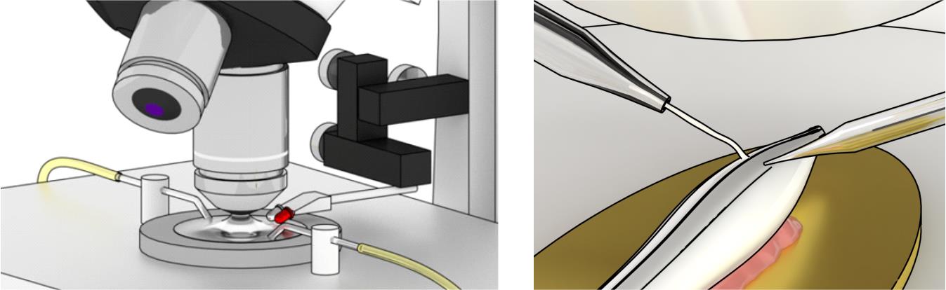
Figure 13. Schematic illustration of the experimental setup. Left: Overview of the experimental setup showing perfusion inflow and outflow tubing, a low-magnification objective, a high-magnification water-immersion objective, and both white and infrared (IR)-LEDs mounted on a micromanipulator. The LEDs should be connected to an adjusted power supply unit and positioned so that their beams strike the plane of the experimental chamber at a 10–20° angle. Note that the LEDs must remain above the bath solution and should not be submerged. Right: Overview of spinal cord preparation in the experimental chamber. The ex vivo spinal cord preparation is affixed to a metal plate at an approximately 45° angle so that the dorsal horn is on top. The spared dorsal root is connected to a suction electrode and is slightly pulled to reveal the underlying dorsal horn. Modified from [17].
6. Identify lamina I. It consists of a relatively sparse population of medium-sized (15–35 μm) neurons—multipolar, fusiform, and pyramidal in shape—located within 10–30 μm from the dorsal horn surface. The boundaries of lamina I are marked by bundles of parallel fibers running in the rostrocaudal direction. The dorsal border is further delineated by fibers of the dorsal roots.
Note: In adult mice, cells can be visualized at depths of up to 40–60 μm, corresponding to the outer layer of lamina II. However, light scattering at this depth compromises the quality of cell visualization, making visually guided patch-clamping more difficult. For practical reasons, we advise performing experiments on lamina I neurons located within 10–30 μm from the dorsal horn surface.
7. Choose an appropriate lamina I neuron for electrophysiological experiments.
Note: Larger lamina I neurons (25–30 μm) tend to offer greater stability during long recordings. However, due to the heterogeneity of the lamina I neuronal population, exclusively selecting large neurons may introduce bias and limit the representativeness of the collected data.
8. Optional: Assess ChR2 expression. Given that the viral construct induces expression of ChR2-EYFP, the EYFP fluorescent signal (excitation: 510 nm, emission: 530 nm) may be used to observe axons and en passant boutons of RVM fibers within the lamina I (see Validation section, Figure 15). However, since lamina I neuronal processes extend ventrally, the absence of fluorescence within a given field of view does not necessarily imply that the observed neurons are not under RVM descending control. We recommend fixing the preparation at the end of the experiment in order to perform a detailed post-hoc analysis of ChR2 expression.
F. Patch-clamping lamina I neuron and establishing whole-cell configuration
1. Power on all equipment: switch on the amplifier, digitizer, constant current stimulator, micromanipulator, and monochromator (for optical stimulation). Launch their respective control software. Set the amplifier to voltage-clamp mode.
2. Prepare the pressure control system: connect the pipette holder to a three-way stopcock using silicone tubing. Attach a 2.5 mL syringe to one port and a mouthpiece (a 1 mL syringe without the plunger) to the other.
3. Prepare the internal solution: thaw a 1 mL aliquot of potassium gluconate intracellular solution. Fill a 1 mL syringe, attach a syringe filter, and connect it to a pipette filler.
Note: Keep the syringe on ice or refrigerated at 4–8 °C throughout the experiment to prevent precipitation of potassium gluconate and/or NaGTP, which may block the pipette tip.
4. Fabricate patch pipettes: use borosilicate glass capillaries and a micropipette puller to produce pipettes suitable for whole-cell recordings.
Note: Refer to the Sutter Pipette Cookbook for detailed guidance on patch pipette fabrication. The pipette tip should be approximately 2 μm in diameter, with a resistance of 3–5 MΩ when filled with potassium gluconate solution.
5. Fill and mount the pipette: fill a pipette with potassium gluconate solution and insert it into the pipette holder connected to the amplifier headstage.
6. Position the pipette under the microscope: raise the water-immersion objective to form a meniscus that accommodates the conical section of the pipette. Introduce the pipette into the solution and bring the tip into focus.
7. Check pipette tip and resistance: visually confirm that the pipette tip is not blocked. Use the Membrane Test (Bath) function in pClamp software to measure pipette resistance, which should be 3–5 MΩ when filled with potassium gluconate.
8. Apply positive pressure: Displace the plunger of the 2.5 mL syringe by 1–1.5 mL to create constant positive pressure. Ensure a visible outflow from the pipette. Compensate for the offset potential.
Note: Applying positive pressure increases the resistance between the patch pipette and the reference electrode by ~0.5–0.7 MΩ when using a potassium gluconate internal solution. A larger increase (several MΩ) typically indicates that the pipette tip is clogged with debris.
9. Approach the surface of the preparation: alternate lowering the objective and the pipette until the tip reaches the surface of the preparation. Then, switch to a fine movement speed on the manipulator and position the tip of the pipette right above the center of the soma of a chosen neuron.
10. Advance toward the cell: slowly descend the pipette toward the neuron. Once the pipette tip enters the tissue, the outward flow of solution should visibly displace and spread the surrounding tissue.
11. Establish gigaseal contact:
Critical: The outflow of high-potassium solution depolarizes nearby neurons. Minimize the time between tissue penetration and gigaseal formation.
a. Continue descending until the cell membrane visibly indents due to pressure.
Note: The solution flow may displace the target cell. Use the manipulator to keep the pipette tip centered over the soma at all times.
b. When the indentation reaches twice the size of the pipette opening, switch the stopcock to the mouthpiece and immediately apply gentle negative pressure (as if sipping through a straw).
c. A sharp increase (to 200–300 MΩ) in pipette resistance should be observed. At this point, release the suction.
d. A gigaseal (≥1 GΩ) should form spontaneously within several seconds. If not, apply gentle negative pressure or negative potential to promote seal formation.
Important:
i. Insufficient indentation prevents gigaseal formation.
ii. Excessive indentation may damage the membrane and prevent successful whole-cell access.
12. Compensate pipette capacitance: once the gigaseal is established, compensate for the pipette capacitance and allow the pipette–cell interface to stabilize for a few minutes. The leak current should be below 20 pA, ideally under 10 pA.
13. Optional: Perform cell-attached recordings to assess the effect of descending modulation on action potential firing of lamina I neurons. Use the stimulation patterns described in section G.
Note: Once the gigaseal is established, only a small patch of the membrane is exposed to the high-potassium solution, so neuronal depolarization is no longer an issue. Cell-attached recordings may be performed in either current (I = 0) or voltage (V = 0) clamp mode. Current-clamp mode allows for detailed analysis of action potential properties, whereas voltage-clamp mode is primarily suited for counting action potentials. For a more comprehensive description of cell-attached recording techniques, see [18].
14. Establish whole-cell patch-clamp configuration:
a. Set the holding potential to -70 mV.
b. To achieve membrane breakthrough, apply gentle negative pressure through the mouthpiece, gradually increasing it until the flat line observed in the Membrane Test (Patch)—indicative of a gigaseal—changes into a characteristic whole-cell transient. Once the transient appears, immediately release the negative pressure.
15. Critical: Continuously monitor the series resistance, as it often increases over time. Higher pipette resistance tends to correlate with greater drift in series resistance. To ensure data quality, do not proceed with recordings if the series resistance changes by more than 20%.
Note: Series resistance varies among cells. Larger lamina I neurons typically show values of 15–25 MΩ, while smaller ones may range from 25 to 35 MΩ. In general, series resistance should be at least an order of magnitude lower than the membrane resistance.
Optional: Compensate the whole-cell transient and series resistance.
G. Electrophysiological recordings, electrical, and ChR2 stimulations
1. Set up the protocols for electrophysiological recordings, dorsal root stimulation, and ChR2 photostimulation.
a. Set the digitization at 10–20 kHz and the Bessel filter at 2.4–3 kHz.
b. Connect the stimulator to the digitizer’s digital output and configure it to deliver square current pulses. Set the stimulation frequency to 0.1 Hz to prevent conduction slowing [19] and avoid the wind-up phenomenon [20]. Set the parameters for dorsal root stimulation [21,22]:
i. 30–50 μA × 50 μs stimuli to activate thick fast-conducting myelinated low-threshold Aβ-fiber primary afferents.
ii. 60–100 μA × 50 μs stimuli to activate Aβ-, thinly myelinated Aδ-, and slow-conducting low-threshold C-fiber primary afferents.
iii. 20–150 μA × 1 ms stimuli to activate all primary afferents, including high-threshold Aβ-, Aδ-, and C-fibers.
iv. -20–150 μA × 1 ms stimuli to exclusively activate C-fiber primary afferents. Negative polarity stimuli are required to induce an anodal block of fast-conducting A fibers [9,15,16,22], thereby ensuring selective activation of C-fibers.
Note: Primary afferent–evoked postsynaptic currents typically reach saturation at 70–100 μA. Therefore, 1 ms stimulation in the 100–150 μA range is considered supramaximal.
c. For ChR2 photostimulation, set the following parameters:
i. Excitation wavelength: 470 nm;
ii. Stimulus duration: 10 ms;
iii Stimulation frequency: 5 Hz.
Optional: Set the triggers to couple photostimulation and electrophysiological recordings.
Note: The photostimulation parameters provided here should be regarded as a reference. Exact values need to be determined experimentally, as they depend on factors such as ChR2 expression levels, light source power, and the optical setup. In our experiments, the light source delivered up to 10 mW of power. Under these conditions, 10 ms pulses at 5 Hz were sufficient to elicit statistically significant effects. Depending on the experimental design, the stimulation frequency can be increased up to 20 Hz.
2. Optional: Within the first minute of achieving whole-cell configuration, run protocols to assess the passive parameters of the membrane and firing properties of the neuron. This data can assist in classifying the recorded cells.
a. To determine membrane resistance and capacitance, apply a -10 mV hyperpolarizing voltage step lasting 200 ms at 1 Hz for 10–15 trials.
b. To characterize the neuronal firing pattern, switch to current-clamp mode and inject a hyperpolarizing current sufficient to bring the membrane potential to -80 mV (to allow recovery of voltage-gated potassium channels from inactivation). Then, apply incrementally increasing 500 ms depolarizing current steps at 0.3 Hz, starting from -20 pA and increasing by 10–20 pA per trial. Avoid exceeding 400–500 pA currents.
3. Verify the series resistance before proceeding to the next recording and adjust it if needed. Do not perform further experiments if the series resistance exceeds 35–40 MΩ. Wait an additional 2–3 min to allow for complete cell dialysis.
4. Critical: Before proceeding to photostimulations, switch to an appropriate optical filter set.
5. Record excitatory postsynaptic currents at a holding potential of -70 mV to assess the effects of photostimulation on network activity and primary afferent input to lamina I neurons.
a. Record spontaneous excitatory postsynaptic currents in gap-free mode for 1–3 min. Then, perform the same recording in the presence of continuous photostimulation, i.e., 10 ms/5 Hz stimulation should be performed throughout the entire recording.
b. After photostimulation, allow 1–2 min for recovery before proceeding with further experiments.
c. Perform desired dorsal root stimulations and register primary afferent–driven excitatory postsynaptic currents. Record at least 12–15 trials for each type of dorsal root stimulation.
d. Perform the same dorsal root stimulations in the presence of continuous photostimulation.
6. Set the holding potential to -10 mV and allow 1–2 min for the baseline current to stabilize.
7. Repeat step G5 to record inhibitory postsynaptic currents and evaluate the impact of photostimulation on inhibitory network activity and primary afferent–driven polysynaptic currents.
Note: Given that the reversal potential for chloride ions is around -80 mV for the combination of external Krebs bicarbonate and internal potassium gluconate solutions, inhibitory currents appear as positive deflections from the baseline.
8. The procedures outlined in steps G5–7 may be repeated in the presence of a pharmacological agent of interest.
Data analysis
The general approach to data analysis involves comparing various parameters of recorded postsynaptic currents under control conditions and during photostimulation.
Spontaneous postsynaptic currents are best analyzed using MiniAnalysis software, which automatically provides the amplitude and kinetics of individual events and calculates interevent intervals.
Analysis of dorsal root stimulation data is best performed using Clampfit or Origin software and involves calculating the integrals of postsynaptic currents and the amplitudes of monosynaptic primary afferent input components. The latter are particularly important: photostimulation-induced decrease in monosynaptic amplitudes directly evidences RVM fiber–dependent presynaptic inhibition of synaptic transmission between primary afferents and lamina I neurons. Studies indicate that the extent of descending modulation differs among different types of primary afferents [9]. Therefore, it is essential to classify monosynaptic inputs accordingly. Monosynaptic components of primary afferent inputs evoked by dorsal root stimulation are identified and classified based on the following criteria [9,21]:
1. Low failure rate, typically less than 30%.
2. Minimal latency variability, with fluctuations of less than 2 ms.
3. Conduction velocity (CV), calculated by dividing the length of the dorsal root (measured from the suction electrode opening to the dorsal root entry zone) by the latency of the monosynaptic response, allowing 1 ms for synaptic transmission:
a. CV < 0.5 m/s corresponds to C-fiber afferents.
b. 0.6–3 m/s corresponds to Aδ-fiber afferents.
c. CV > 3.5 m/s corresponds to Aβ-fiber afferents.
Datasets obtained from described experiments often deviate from a normal distribution. Therefore, nonparametric statistical tests are recommended for comparisons. We recommend using the Mann–Whitney test for statistical comparisons of postsynaptic current integrals and monosynaptic primary afferent input amplitudes. For larger datasets derived from the analysis of spontaneous postsynaptic currents, the Kolmogorov–Smirnov test is more appropriate.
For presentation purposes, traces can be mildly smoothed using a Savitzky–Golay filter to reduce high-frequency noise caused by the peristaltic pump.
Validation of protocol
To characterize the spatiotemporal pattern of expression, we injected an AAV9-hSyn-EGFP viral construct (50 nL) into the RVM. Five to seven weeks later, the brains and spinal cords were fixed, sectioned, and examined using a confocal microscope. EGFP fluorescence was detected in both the RVM and the spinal cord (Figure 14A–D). Within the spinal cord, the strongest EGFP signal was observed in the dorsolateral funiculus, the known pathway of RVM-originating fibers. In the spinal gray matter, the highest signal intensity was detected in the superficial dorsal horn (laminae I–II) and around the central canal (lamina X)—regions involved in the processing of nociceptive information. EGFP expression remained consistent between weeks 5 and 7 after stereotaxic injection, with no significant differences in signal intensity. Neither the sex of the experimental mice nor an increased injection volume (100 and 150 nL vs 50 nL) had a significant effect on EGFP expression.
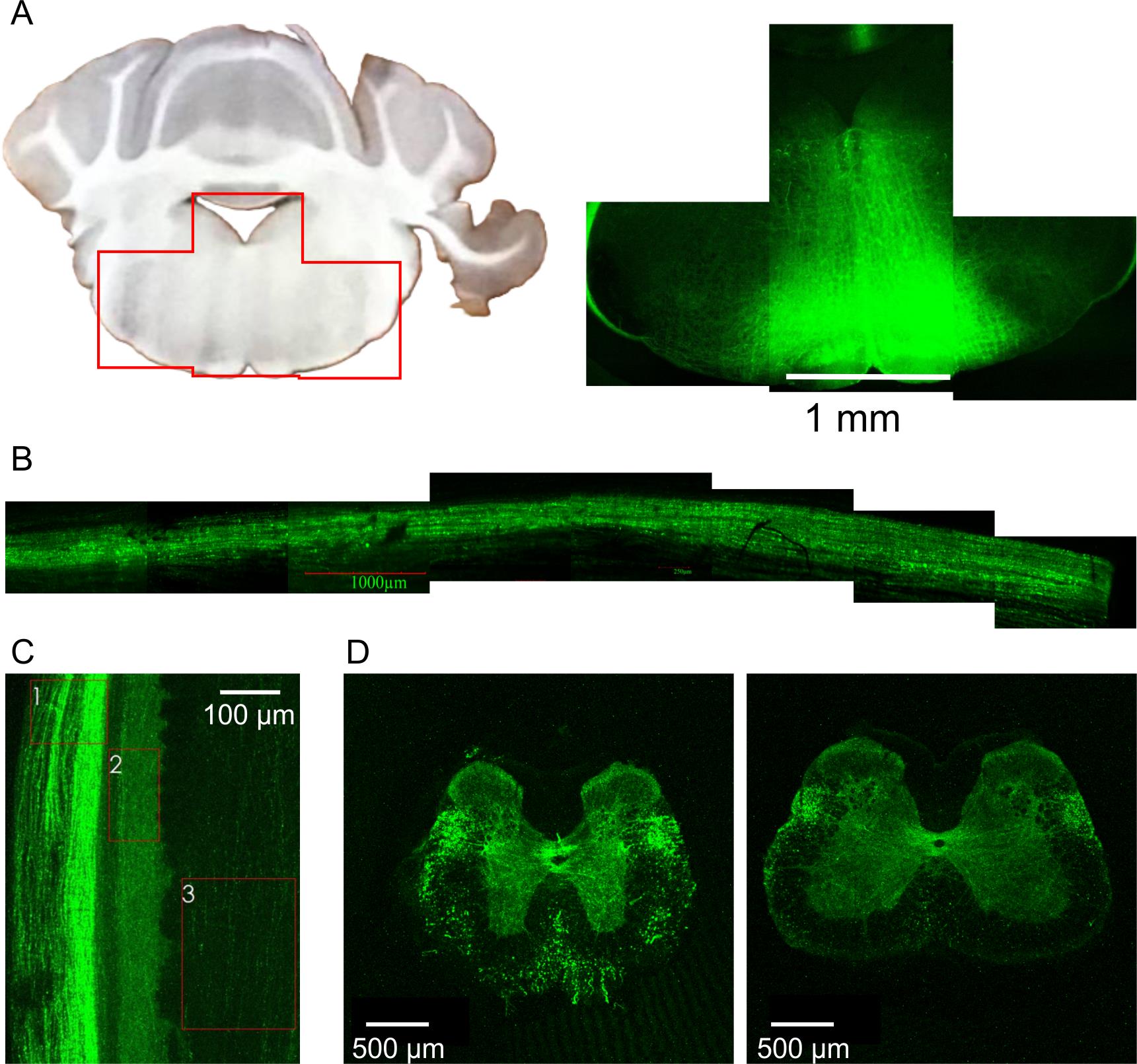
Figure 14. EGFP expression patterns after stereotaxic injection of the respective viral construct into the rostral ventromedial medulla (RVM). (A) Expression of EGFP within the RVM. (B) EGFP fluorescent signal from the dorsolateral funiculus of the spinal cord. (C, D) EGFP expression pattern in the spinal cord. (C) Lateral view of the spinal cord. 1: dorsolateral funiculus; 2: lamina I; 3: dorsal column. (D) Coronal sections showing EGFP fluorescence in the thoracic (left) and lumbar (right) segments. Notice that the highest intensity of EGFP signal is observed for the dorsolateral funiculus, superficial dorsal horn (lamina I–II), and the area around the central canal (lamina X).
The expression pattern of channelrhodopsin-2 (ChR2–EYFP) following stereotaxic injection of the corresponding viral construct into the RVM closely matched that of EGFP. Spinal lamina I exhibited intense ChR2–EYFP fluorescence, revealing a dense network of labeled fibers interspersed with prominent en passant boutons (Figure 15).
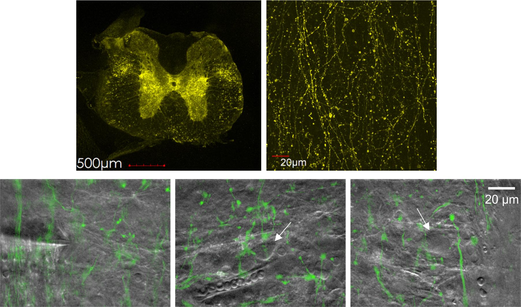
Figure 15. Channelrhodopsin-2 (ChR2)–EYFP expression pattern in the spinal cord. Top row: Confocal images showing ChR2–EYFP expression in the spinal cord (left) and in spinal lamina I (right). Bottom row: infrared (IR)-LED oblique illumination images (gray) overlaid with epifluorescent ChR2–EYFP images (green), revealing rostral ventromedial medulla (RVM)-originating fibers and en passant boutons. White arrows indicate somata of lamina I neurons. Notice a patched neuron in the left image.
To assess the effectiveness of ChR2 photostimulation, we performed patch-clamp recordings from lumbar lamina I neurons. We first examined primary afferent–driven postsynaptic currents evoked by electrical dorsal root stimulation. Continuous (5 Hz) ChR2 photostimulation significantly reduced excitatory (recorded at -70 mV holding potential) and inhibitory (recorded at -10 mV) postsynaptic currents (Figure 16A, B) in 4 of 5 and 3 of 4 tested neurons, respectively, suggesting that RVM could both inhibit and facilitate nociception. In 2 out of 5 tested neurons, photostimulation also diminished the monosynaptic component of primary afferent input, indicating its presynaptic inhibition by RVM-originating descending fibers (Figure 16A). Next, we performed gap-free recordings to assess photostimulation-induced postsynaptic activity. In 2 of the 10 tested neurons, we observed bursts of inhibitory postsynaptic currents in response to photostimulation (Figure 16C). These bursts were synchronized, with the first event exhibiting low jittering (1–3 ms), suggesting the presence of direct synaptic contacts between lamina I neurons and RVM-originating fibers.
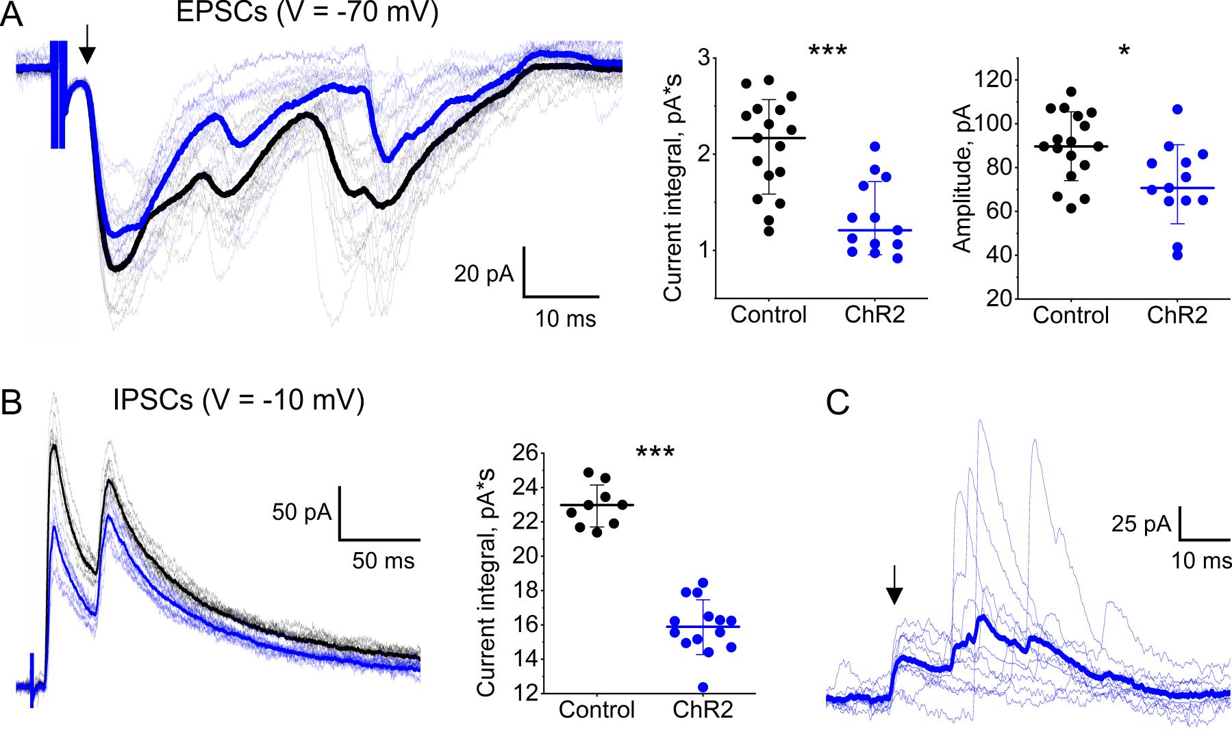
Figure 16. Effects of channelrhodopsin-2 (ChR2) photostimulation of rostral ventromedial medulla (RVM) fibers on synaptic activity of lamina I neurons. (A, B) ChR2 photostimulation-induced reduction of primary afferent–driven postsynaptic currents. (A) Left: Patch-clamp recordings of excitatory postsynaptic currents (EPSCs) evoked by electrical dorsal root stimulation. Black traces: no photostimulation. Blue traces: continuous (5 Hz, 10 ms pulses) ChR2 photostimulation. Thick curves: averaged traces. The arrow indicates A-fiber-driven monosynaptic component of primary afferent input. Effects of ChR2 photostimulation on the EPSC integral (middle) and on the amplitude of the monosynaptic component (right). (B) Left: Patch-clamp recordings of inhibitory postsynaptic currents (IPSCs) evoked by electrical dorsal root stimulation. Black traces: no photostimulation. Blue traces: continuous ChR2 photostimulation (5 Hz, 10 ms pulses). Thick curves: averaged traces. Right: Effect of ChR2 photostimulation on the IPSC integral. (C) Postsynaptic inhibitory currents elicited in response to 10 consecutive light pulses. Blue traces: individual IPSCs evoked by ChR2 photostimulation of RVM fibers. Thick blue curve: an averaged trace. An arrow indicates a presumable monosynaptic component of IPSCs. *p < 0.05, ***p < 0.001, Mann–Whittney test.
Overall, these data provide compelling evidence that our methodological approach can be used for investigating pre- and postsynaptic mechanisms of RVM-dependent descending modulation.
Sections of this protocol detailing ex vivo spinal cord preparation and electrophysiological recordings from lamina I neurons combined with dorsal root stimulations have been used and validated in the following research articles:
• Krotov et al. [16]. Elucidating afferent-driven presynaptic inhibition of primary afferent input to spinal laminae I and X. Frontiers in Cellular Neuroscience.
• Krotov et al. [23]. Neuropathic pain changes the output of rat lamina I spino-parabrachial neurons. BBA Advances.
• Tadokoro et al. [24]. Precision spinal gene delivery-induced functional switch in nociceptive neurons reverses neuropathic pain. Molecular Therapy.
• Agashkov and Krotov et al. [25]. Distinct mechanisms of signal processing by lamina I spino-parabrachial neurons. Scientific Reports.
• Krotov et al. [26]. High-threshold primary afferent supply of spinal lamina X neurons. Pain.
• Krotov et al. [9]. Segmental and descending control of primary afferent input to the spinal lamina X. Pain.
General notes and troubleshooting
General notes
1. This protocol can be applied to investigate RVM-dependent descending modulation in various pain models, including complete Freund’s adjuvant-induced peripheral inflammation, spared nerve injury-induced neuropathy, etc.
2. This protocol could be easily adapted for studying descending modulation mediated by other supraspinal structures, such as dorsal reticular and parabrachial nuclei.
3. This protocol could greatly benefit from incorporating approaches and techniques for labeling specific neuronal populations.
a. The use of transgenic mice with GFP tag expressed under different promoters [27] could reveal RVM-dependent descending modulation of glutamate-, GABA-, and glycinergic lamina I neurons.
b. Retrograde labeling using Fluorogold [25] could allow the study of descending modulation of lamina I projection neurons, a specific population that transmits nociceptive information from the spinal cord to supraspinal centers.
4. Electrophysiological recordings from lamina I neurons could be combined with Ca2+ transient measurements using both membrane-impermeable and genetically encoded red fluorescent Ca2+ indicators.
5. This protocol may be adapted for use in young rats. However, since lamina I recordings are only feasible in rats younger than P30, this would necessitate stereotaxic targeting of the RVM in neonatal rats (P5–P7), which presents a significant technical challenge.
Troubleshooting
We acknowledge that this protocol is lengthy, complex, and requires skilled personnel for successful execution. Therefore, we strongly recommend practicing and mastering each section of the procedure separately before attempting the entire protocol as a whole.
The most technically demanding step is the ex vivo spinal cord preparation. Even for experienced experimenters, the success rate typically does not exceed 90%. Common pitfalls include accidental severing of dorsal roots, incomplete removal of the meninges, and inadequate adhesion of the preparation to the metal plate. Unfortunately, these errors are irreversible and render the preparation unusable.
Given these challenges, it is important to account for potential losses when planning and designing experiments.
Acknowledgments
Author contributions: V.K., conceptualization, investigation, writing—original draft, writing—review & editing; I.B., J.M., A.M., and S.R., investigation; N.V. and P.B., conceptualization, funding acquisition, supervision.
This work was supported by NIH/NINDS grant NS113189 and the National Academy of Science of Ukraine grants 0124U001556 and 0124U001557.
Parts of this protocol have been previously used and validated in the following research articles: [9,16,23–26].
The authors acknowledge the use of generative AI (ChatGPT 4.0) to improve the clarity and readability of the text. All authors reviewed the edited version and confirmed that it accurately reflects their views.
The authors thank Dr. Andrew Dromaretsky (Bogomoletz Institute of Physiology) for technical assistance.
Competing interests
The authors declare no conflicts of interest.
Ethical considerations
All procedures involving animals were carried out with the approval of the Animal Ethics Committee of the Bogomoletz Institute of Physiology (Kyiv, Ukraine) in accordance with the European Commission Directive (86/609/EEC), ethical guidelines of the International Association for the Study of Pain, and the Society for Neuroscience Policies on the Use of Animals and Humans in Neuroscience Research.
References
- Safronov, B. V. and Szucs, P. (2024). Novel aspects of signal processing in lamina I. Neuropharmacology. 247: 109858. https://doi.org/10.1016/j.neuropharm.2024.109858
- Todd, A. J. (2010). Neuronal circuitry for pain processing in the dorsal horn. Nat Rev Neurosci. 11(12): 823–836. https://doi.org/10.1038/nrn2947
- Bannister, K. (2019). Descending pain modulation: influence and impact. Curr Opin Physiol. 11: 62–66. https://doi.org/10.1016/J.COPHYS.2019.06.004
- Ossipov, M. H., Morimura, K. and Porreca, F. (2014). Descending pain modulation and chronification of pain. Curr Opin Support Palliat Care. 8(2): 143. https://doi.org/10.1097/SPC.0000000000000055
- Ossipov, M. H., Dussor, G. O. and Porreca, F. (2010). Central modulation of pain. J Clin Invest. 120(11): 3779–3787. https://doi.org/10.1172/JCI43766
- Fitzgerald, M. and Koltzenburg, M. (1986). The functional development of descending inhibitory pathways in the dorsolateral funiculus of the newborn rat spinal cord. Dev Brain Res. 24: 261–270. https://doi.org/10.1016/0165-3806(86)90194-x
- Behbehani, M. M. and Zemlan, F. P. (1990). Bulbospinal and intraspinal thyrotropin releasing hormone systems: modulation of spinal cord pain transmission. Neuropeptides. 15(3): 161–168. https://doi.org/10.1016/0143-4179(90)90149-S
- Ness, T. J. and Gebhart, G. F. (1987). Quantitative comparison of inhibition of visceral and cutaneous spinal nociceptive transmission from the midbrain and medulla in the rat. J Neurophysiol. 58(4): 850–865. https://doi.org/10.1152/JN.1987.58.4.850
- Krotov, V., Agashkov, K., Krasniakova, M., Safronov, B. V, Belan, P. and Voitenko, N. (2022). Segmental and descending control of primary afferent input to the spinal lamina X. Pain. 163(10): 2014–2020. https://doi.org/10.1097/j.pain.0000000000002597
- François, A., Low, S. A., Sypek, E. I., Christensen, A. J., Sotoudeh, C., Beier, K. T., Ramakrishnan, C., Ritola, K. D., Sharif-Naeini, R., Deisseroth, K., et al. (2017). A Brainstem-Spinal Cord Inhibitory Circuit for Mechanical Pain Modulation by GABA and Enkephalins. Neuron. 93(4): 822–839.e6. https://doi.org/10.1016/J.NEURON.2017.01.008
- Safronov, B. V., Pinto, V. and Derkach, V. A. (2007). High-resolution single-cell imaging for functional studies in the whole brain and spinal cord and thick tissue blocks using light-emitting diode illumination. J Neurosci Methods. 164(2): 292–298. https://doi.org/10.1016/j.jneumeth.2007.05.010
- Szűcs, P., Pinto, V. and Safronov, B. V. (2009). Advanced technique of infrared LED imaging of unstained cells and intracellular structures in isolated spinal cord, brainstem, ganglia and cerebellum. J Neurosci Methods. 177(2): 369–380. https://doi.org/10.1016/j.jneumeth.2008.10.024
- Krotov, V., Belan, P. and Voitenko, N. (2024). Approach for Electrophysiological Studies of Spinal Lamina X Neurons. Bio Protoc. 14(14): e5035. https://doi.org/10.21769/BIOPROTOC.5035
- Krotov, V. and Kopach, O. (2024). Nerve Preparation and Recordings for Pharmacological Tests of Sensory and Nociceptive Fiber Conduction Ex Vivo. Bio Protoc. 14(7): e4969. https://doi.org/10.21769/BIOPROTOC.4969
- Fernandes, E. C., Pechincha, C., Luz, L. L., Kokai, E., Szucs, P. and Safronov, B. V. (2020). Primary afferent-driven presynaptic inhibition of C-fiber inputs to spinal lamina I neurons. Prog Neurobiol. 188: 101786. https://doi.org/10.1016/j.pneurobio.2020.101786
- Krotov, V., Agashkov, K., Romanenko, S., Halaidych, O., Andrianov, Y., Safronov, B. V., Belan, P. and Voitenko, N. (2023). Elucidating afferent-driven presynaptic inhibition of primary afferent input to spinal laminae I and X. Front Cell Neurosci, 16, 670. https://doi.org/10.3389/FNCEL.2022.1029799/BIBTEX
- Krotov, V., Tokhtamysh, A., Kopach, O., Dromaretsky, A., Sheremet, Y., Belan, P. and Voitenko, N. (2017). Functional Characterization of Lamina X Neurons in ex-Vivo Spinal Cord Preparation. Front Cell Neurosci. 11: 342. https://doi.org/10.3389/fncel.2017.00342
- Perkins, K. L. (2006). Cell-attached voltage-clamp and current-clamp recording and stimulation techniques in brain slices. J Neurosci Methods. 154(1–2): 1. https://doi.org/10.1016/J.JNEUMETH.2006.02.010
- Pinto, V., Derkach, V. A. and Safronov, B. V. (2008). Role of TTX-Sensitive and TTX-Resistant Sodium Channels in Aδ- and C-Fiber Conduction and Synaptic Transmission. J Neurophysiol. 99(2): 617–628. https://doi.org/10.1152/JN.00944.2007
- Hachisuka, J., Omori, Y., Chiang, M. C., Gold, M. S., Koerber, H. R. and Ross, S. E. (2018). Wind-up in lamina I spinoparabrachial neurons. Pain. 159(8): 1484–1493. https://doi.org/10.1097/j.pain.0000000000001229
- Luz, L. L., Szucs, P. and Safronov, B. V. (2014). Peripherally driven low-threshold inhibitory inputs to lamina I local-circuit and projection neurones: a new circuit for gating pain responses. J Physiol. 592(7): 1519–1534 https://doi.org/10.1113/jphysiol.2013.269472
- Luz, L. L., Lima, S., Fernandes, E. C., Kokai, E., Gomori, L., Szucs, P. and Safronov, B. V. (2023). Contralateral Afferent Input to Lumbar Lamina I Neurons as a Neural Substrate for Mirror-Image Pain. J Neurosci. 43(18): 3245–3258. https://doi.org/10.1523/JNEUROSCI.1897-22.2023
- Krotov, V., Agashkov, K., Romanenko, S., Koroid, K., Krasniakova, M., Belan, P. and Voitenko, N. (2023). Neuropathic pain changes the output of rat lamina I spino-parabrachial neurons. BBA Adv. 3. https://doi.org/10.1016/J.BBADVA.2023.100081
- Tadokoro, T., Bravo-Hernandez, M., Agashkov, K., Kobayashi, Y., Platoshyn, O., Navarro, M., Marsala, S., Miyanohara, A., Yoshizumi, T., Shigyo, M., et al. (2022). Precision spinal gene delivery-induced functional switch in nociceptive neurons reverses neuropathic pain. Molecular Therapy. 30(8): 2722–2745. https://doi.org/10.1016/J.YMTHE.2022.04.023
- Agashkov, K., Krotov, V., Krasniakova, M., Shevchuk, D., Andrianov, Y., Zabenko, Y., Safronov, B. V., Voitenko, N. and Belan, P. (2019). Distinct mechanisms of signal processing by lamina I spino-parabrachial neurons. Sci Rep. 9(1): 1–12. https://doi.org/10.1038/s41598-019-55462-7
- Krotov, V., Tokhtamysh, A., Safronov, B. V, Belan, P. and Voitenko, N. (2019). High-threshold primary afferent supply of spinal lamina X neurons. Pain. 160(9): 1982–1988. https://doi.org/10.1097/j.pain.0000000000001586
- Punnakkal, P., von Schoultz, C., Haenraets, K., Wildner, H. and Zeilhofer, H. U. (2014). Morphological, Biophysical and Synaptic Properties of Glutamatergic Neurons of the Mouse Spinal Dorsal Horn. J Physiol. 592(4): 759–776. https://doi.org/10.1113/jphysiol.2013.264937
Article Information
Publication history
Received: Aug 18, 2025
Accepted: Sep 18, 2025
Available online: Oct 10, 2025
Published: Nov 5, 2025
Copyright
© 2025 The Author(s); This is an open access article under the CC BY-NC license (https://creativecommons.org/licenses/by-nc/4.0/).
How to cite
Krotov, V., Blashchak, I., Moore, J., Moore, A., Romanenko, S., Voitenko, N. and Belan, P. (2025). Optogenetic Approach for Investigating Descending Control of Nociception in Ex Vivo Spinal Cord Preparation. Bio-protocol 15(21): e5483. DOI: 10.21769/BioProtoc.5483.
Category
Neuroscience > Sensory and motor systems > Spinal cord
Systems Biology > Connectomics > Cellular connectivity
Do you have any questions about this protocol?
Post your question to gather feedback from the community. We will also invite the authors of this article to respond.