- Protocols

- Articles and Issues
- For Authors
- About
- Become a Reviewer

Advancing 2-DE Techniques: High-Efficiency Protein Extraction From Lupine Roots
Published: Vol 15, Iss 19, Oct 5, 2025 DOI: 10.21769/BioProtoc.5461 Views: 1791
Reviewed by: Nicolás M. CecchiniSamik Bhattacharya

Protocol Collections
Comprehensive collections of detailed, peer-reviewed protocols focusing on specific topics


Related protocols
Abstract
Protein isolation combined with two-dimensional electrophoresis (2-DE) is a powerful technique for analyzing complex protein mixtures, enabling the simultaneous separation of thousands of proteins. This method involves two distinct steps: isoelectric focusing (IEF), which separates proteins based on their isoelectric points (pI), and sodium dodecyl sulfate–polyacrylamide gel electrophoresis (SDS-PAGE), which separates proteins by their relative molecular weights. However, the success of 2-DE is highly dependent on the quality of the starting material. Isolating proteins from plant mature roots is challenging due to interfering compounds and a thick, lignin-rich cell wall. Bacterial proteins and metabolites further complicate extraction in legumes, which form symbiotic relationships with bacteria. Endogenous proteases can degrade proteins, and microbial contaminants may co-purify with plant proteins. Therefore, comparing extraction methods is essential to minimize contaminants, maximize yield, and preserve protein integrity. In this study, we compare two protein isolation techniques for lupine roots and optimize a protein precipitation protocol to enhance the yield for downstream proteomic analyses. The effectiveness of each method was evaluated based on the quality and resolution of 2-DE gel images. The optimized protocol provides a reliable platform for comparative proteomics and functional studies of lupine root responses to stress, e.g., drought or salinity, and symbiotic interactions with bacteria.
Key features
• Protocol tailored for isolating proteins from lupine roots, including those involved in symbiotic relationships with bacteria.
• Our method is suitable for analyzing complex protein mixtures through IEF and SDS-PAGE for high-resolution separation.
• Optimized precipitation method increases protein yield for downstream mass spectrometry and comparative proteomic analyses.
Keywords: Protein isolationBackground
Proteomic analyses are crucial in plant physiology research, providing valuable insight into plant function. However, these studies' success heavily depends on the quantity and quality of the extracted material. Proteins play key roles in enzymatic activity, signaling, and defense, directly influencing plant health and its interactions with the surrounding ecosystem. This is especially significant for roots, which are essential for nutrient uptake and transport. Despite their importance, isolating proteins from mature roots presents several technical challenges that limit progress in proteomic and biochemical analyses. Traditional protein isolation protocols, typically designed for leaf or seed tissues, are often ineffective for roots, due to their distinct biochemical composition, unique physiology, and lower protein content compared to aboveground tissues [1]. Therefore, it becomes necessary to adapt homogenization methods, select appropriate extraction buffers containing protease inhibitors, and optimize purification techniques.
One of the major challenges in isolating proteins from plant roots is the presence of phenolic compounds, which, upon oxidation, form stable complexes with proteins, thereby reducing their recovery [2,3]. Other significant issues include the increased rigidity of the cell walls, which impede homogenization, as well as the presence of polysaccharides and other carbohydrates that increase sample viscosity. Additionally, certain compounds such as detergents, salts, or lipids may interfere with protein extraction and co-precipitate with the proteins of interest [4,5]. Root tissue is also characterized by high endogenous proteolytic activity, which can lead to rapid protein degradation during homogenization and subsequent extraction steps [3,4]. This degradation is especially pronounced when cell structures are disrupted, causing proteases to be released from their native compartments. To mitigate this, the use of protease inhibitors, such as phenylmethylsulfonyl fluoride (PMSF) or commercially available inhibitor mixtures, is critical. In legumes, where specific bacterial proteases are present due to a symbiotic relationship with Rhizobium bacteria, additional cysteine protease inhibitors may be required [6]. Furthermore, the entire procedure should be conducted at the lowest possible temperature to reduce enzymatic activity, and the protein isolation process should be performed as quickly as possible to minimize the exposure of proteins to proteases [3,4]. In some cases, pre-purification of samples using trichloroacetic acid (TCA)/acetone protein precipitation can be beneficial, as it helps to inactivate certain proteolytic enzymes. This method, originally developed by Damerval et al. [7] and later modified by Saravanan and Rose [8], Isaacson et al. [3], and Fic et al. [9], is widely applied to various tissues. It is important to note that prolonged exposure of the extract to acetone can negatively affect protein structure, which may, in turn, compromise the result of MS/MS analysis at later stages [10]. Additionally, protein degradation can occur due to prolonged exposure to low pH [4,11]. To mitigate this, an aqueous TCA solution is often used for precipitation [12], although the resulting proteins may be more challenging to solubilize.
Given the critical role of proteomic research in understanding plant physiology and the stringent requirements regarding the quantity and purity of protein material, it is essential to continually adapt methods to meet the specific needs of the plant tissue being studied. This is especially important for economically significant species, such as yellow lupine (Lupinus luteus L.), where the quality and yield of protein extraction directly impact research outcomes and practical applications. In the context of the European Union’s pro-environmental policies, this species is recognized as a natural source of nitrogen (N2), fixed from the atmosphere through symbiosis with Bradyrhizobium bacteria. This process reduces the need for synthetic fertilizers, thereby minimizing environmental impact. Additionally, N2 fixed in this way is stored in the soil, making it less prone to leaching by precipitation. Studying the proteome offers valuable insight into these processes, enabling the identification of proteins involved in the plant's response to various environmental conditions. This research will advance our current understanding of plant N2 fixation and its broader ecological implications. The challenge of isolating proteins from yellow lupine roots was previously addressed by Orzoł and Piotrowicz-Cieślak [13] through their study focused on seedlings at early developmental stages up to 12 days. The authors performed analyses on young plants that had not yet developed nodules and contained lower levels of secondary metabolites, which could affect isolation efficiency. This study aims to compare two commonly used protein isolation methods for obtaining root material from lupine suitable for two-dimensional electrophoresis. Additionally, we have optimized a protein precipitation method to increase the yield of material for proteomic analyses. The effectiveness of each method was assessed by comparing 2-DE PAGE gel images of the resulting protein samples. Our optimization assay identified the Tris-EDTA protocol as the most effective protein isolation method, with a 1-h TCA/acetone precipitation step yielding the highest protein recovery.
Materials and reagents
Biological materials
1. Commercial yellow lupine cultivar Taper was grown in phytotron chambers under controlled conditions, as optimized previously by Frankowski et al. [14]. In brief, seeds were sourced from Poznań Plant Breeding Tulce (Wiatrowo, Poland), treated with Sarfun (2.5 mL per kg of seeds; Organika-Sarzyna S.A., Nowa Sarzyna, Poland), and inoculated for 2 h with Nitragina (3 g per kg of seeds, BIOFOOD S.C., Wałcz, Poland). Seeds were then sown into pots filled with class V field soil (53° 6' 22.383" N 18° 27' 1.922" E) and grown at 22 °C ± 1 °C under long day conditions (16 h light/8 h dark, 110 μmol m-2 s-1 cool white fluorescent lighting; Polam, Warsaw, Poland). On day 48 of cultivation, roots were harvested as described by Burchardt et al. [15]. The root system was divided into two distinct zones: an upper region bearing nitrogen-fixing nodules, and a lower, nodule-free region. For this study, nodules were removed from the upper root segment, and the remaining tissue was frozen in liquid nitrogen and stored at -80 °C for further analysis.
Reagents
1. Phenol solution, BioReagent, equilibrated with 10 mM Tris HCl, pH 8.0, 1 mM ethylenediaminetetraacetic acid (EDTA), for molecular biology (Sigma-Aldrich, Merck KGaA, catalog number: P4557)
2. Sodium dodecyl sulfate (SDS) (Sigma-Aldrich, Merck KGaA, catalog number: 11667289001)
3. Sucrose, molecular biology grade (Milipore, Merck KGaA, catalog number: 573113)
4. β-Mercaptoethanol (Sigma-Aldrich, Merck KGaA, catalog number: M6250)
5. Trizma® base, ≥99.9% (titration), crystalline (Sigma-Aldrich, Merck KGaA, catalog number: T4661)
6. Hydrochloric acid (HCl) 37%, ACS reagent (Sigma-Aldrich, Merck KGaA, catalog number: 258148)
7. PMSF (Roche, F. Hoffmann-La Roche AG, catalog number: PMSF-RO)
8. Ammonium acetate (Chempur, POL-AURA, catalog number: 111392705)
9. Methanol, anhydrous for analysis (max. 0.003% H2O) (Supelco, Merck KGaA, catalog number: 106012)
10. Acetone suitable for HPLC, ≥99,9% (Sigma-Aldrich, Merck KGaA, catalog number: 270725)
11. Trichloroacetic acid (TCA), ACS reagent (Sigma-Aldrich, Merck KGaA, catalog number: T6399)
12. Ethyl alcohol, pure, ≥99.5%, ACS reagent, 200 proof (Sigma-Aldrich, Merck KGaA, catalog number: 459844)
13. EDTA (Sigma-Aldrich, Merck KGaA, catalog number: E6758)
14. NaCl pure p.a. (Avantor Performance Materials Poland S.A., catalog number: PA-06-794121116)
15. Urea, powder, BioReagent, for molecular biology, suitable for cell culture (Sigma-Aldrich, Merck KGaA, catalog number: U5378)
16. Thiourea, ACS reagent, ≥99.0% (Sigma-Aldrich, Merck KGaA, catalog number: T8656)
17. 3-[(3-Cholamidopropyl)dimethylammonio]-1-propanesulfonate (CHAPS) (Roche, F. Hoffmann-La Roche AG, catalog number: CHAPS-RO)
18. Bovine serum albumin (BSA), lyophilized powder, BioReagent, suitable for cell culture (Sigma-Aldrich, Merck KGaA, catalog number: A9418)
19. Bradford reagent (Supelco, Merck KGaA, catalog number: B6916)
20. Ammonium persulfate (APS), BioXtra, ≥98.0% (Sigma-Aldrich, Merck KGaA, catalog number: A7460)
21. Acetic acid 99.5%–99.9% PURE (Avantor Performance Materials Poland S.A., catalog number: PA-06-568760114)
22. Coomassie Brilliant Blue R-250 protein stain powder (Bio-Rad Laboratories, Inc., catalog number: 1610400)
23. 30% Acrylamide/Bis Solution, 29:1 (Bio-Rad Laboratories, Inc., catalog number: 1610156)
24. N,N,N′,N′-tetramethylethylenediamine (TEMED) (Sigma-Aldrich, Merck KGaA, catalog number: T9281)
25. Glycine (Sigma-Aldrich, Merck KGaA, catalog number: G7126)
26. Protein molecular weight marker PageRulerTM Prestained Protein Ladder, 10–180 kDa (Thermo Fisher Scientific Inc., catalog number: 26617)
27. ReadyPrep 2-D Starter Kit 2-D Gel Electrophoresis kit (Bio-Rad Laboratories, Inc., catalog number: 1632105)
28. ReadyStrip IPG strips 7 cm, pH 3–10 nonlinear (Bio-Rad Laboratories, Inc., catalog number: 1632002)
29. Mineral oil (Bio-Rad Laboratories, Inc., catalog number: 1632129)
Solutions
A. For the phenol method
1. 100 mM Tris-HCl, pH 8.0 (see Recipes)
2. SDS buffer (see Recipes)
3. 100 mM ammonium acetate in methanol (see Recipes)
4. Anhydrous methanol containing 0.1% (w/v) ammonium acetate (see Recipes)
5. 80% (v/v) acetone (see Recipes)
B. For the modified Tris-EDTA method
1. 50 mM Tris-HCl buffer, pH 7.5 (see Recipes)
2. 20% (w/v) TCA in acetone (see Recipes)
3. 20% (w/v) TCA in H2O (see Recipes)
4. 1:1 (v/v) mixture of ethanol and ethyl acetate (see Recipes)
C. Common solutions
1. 1.5 M Tris-HCl, pH 8.8 (see Recipes)
2. 10% (w/v) SDS (see Recipes)
3. 10% (w/v) APS (see Recipes)
4. 7 M urea, 2 M thiourea, 4% (w/v) CHAPS (see Recipes)
5. Bradford assay (see Recipes)
6. 12% (w/v) polyacrylamide gel (see Recipes)
7. 1× SDS-PAGE running buffer (see Recipes)
8. Gel staining solution (see Recipes)
9. Gel destaining solution (see Recipes)
Recipes
A. For the phenol method (based on Wang et al. [4] with modifications of Nisar et al. [16])
1. 100 mM Tris-HCl, pH 8.0
| Reagent | Final concentration | Quantity or volume |
|---|---|---|
| Trizma base | 100 mM | 1.21 g |
| H2O (MilliQ) | n/a | up to 100 mL |
a. Weigh the appropriate amount of Trizma base and transfer it to a bottle.
b. Add 70 mL of H2O (MilliQ) and insert a stirring rod in a bottle.
c. Place the bottle on a magnetic stirrer set to approximately 400 rpm and stir until the Trizma base is fully dissolved.
d. Then insert the pH meter electrode and, while stirring, gradually add HCl in small portions to adjust the pH to 8.0.
e. After reaching the desired pH, dilute the solution with H2O (MilliQ) to a final volume of 100 mL and mix thoroughly. Store the prepared solution at 4 °C for up to 4 weeks.
2. SDS buffer
| Reagent | Final concentration | Quantity or volume |
|---|---|---|
| SDS | 2% | 2 g |
| Sucrose | 30% | 30 g |
| PMSF | 1 mM | 17.42 mg |
| β-mercaptoethanol | 5% | 5 mL |
| 100 mM Tris-HCl, pH 8.0 | 100 mM | up to 100 mL |
a. Weigh the appropriate amounts of the ingredients.
b. Since PMSF is insoluble in water, dissolve it in approximately 5 mL of ethanol, methanol, or isopropanol.
c. Transfer all ingredients to a bottle and add 70 mL of 100 mM Tris-HCl, pH 8.0.
d. Mix until all components are dissolved, then add 5 mL of β-mercaptoethanol. Adjust the volume to 100 mL with 100 mM Tris-HCl, pH 8.0, and mix thoroughly. Store the buffer at 4 °C for up to 4 weeks.
3. 100 mM ammonium acetate in methanol
| Reagent | Final concentration | Quantity or volume |
|---|---|---|
| Ammonium acetate | 100 mM | 1.54 g |
| Anhydrous methanol | 100% | up to 200 mL |
a. Weigh 1.5416 g of ammonium acetate and transfer it to a bottle.
b. Add 150 mL of anhydrous methanol and mix thoroughly.
c. Adjust the volume to 200 mL with methanol and mix again. Store the solution at 4 °C for up to 4 weeks.
4. Anhydrous methanol with 0.1% (w/v) ammonium acetate
| Reagent | Final concentration | Quantity or volume |
|---|---|---|
| Ammonium acetate | 0.1% | 100 mg |
| Anhydrous methanol | 100% | up to 100 mL |
a. Weigh 100 mg of ammonium acetate and transfer it to a bottle.
b. Add 80 mL of anhydrous methanol and mix thoroughly until fully dissolved.
c. Adjust the volume to 100 mL with methanol and mix again.
d. Store the solution at 4 °C for up to 4 weeks.
5. 80% (v/v) acetone
| Reagent | Final concentration | Volume |
|---|---|---|
| Acetone | 80% | 80 mL |
| H2O (MilliQ) | n/a | up to 100 mL |
a. Measure 80 mL of acetone in a cylinder, then add H2O (MilliQ) to bring the total volume to 100 mL.
b. Transfer the solution to a bottle and mix thoroughly.
c. Store at room temperature for up to 6 months.
B. For the modified Tris-EDTA method (based on Azri et al. [17])
1. 50 mM Tris-HCl buffer, pH 7.5
| Reagent | Final concentration | Quantity or volume |
|---|---|---|
| Trizma base | 50 mM | 605.7 mg |
| EDTA | 2 mM | 58.45 mg |
| PMSF | 1 mM | 17.42 mg |
| H2O (MilliQ) | n/a | up to 100 mL |
a. Weigh all required ingredients and transfer them to a clean bottle.
b. As PMSF is not water-soluble, dissolve the measured amount in 5 mL of ethanol.
c. Add 70 mL of H2O (MilliQ) to the bottle and place the solution on a magnetic stirrer.
d. Adjust the pH to 7.5 using HCl while stirring.
e. Once the pH is stabilized, top up the volume to 100 mL with H2O (MilliQ) and mix thoroughly.
f. Store the solution at 4 °C for up to 3 weeks.
2. 20% (w/v) TCA in acetone
| Reagent | Final concentration | Quantity or volume |
|---|---|---|
| TCA | 20% | 20 g |
| Acetone | 100% | up to 100 mL |
a. Weigh the required amount of TCA and dissolve it in 50 mL of acetone.
b. Mix thoroughly until fully dissolved.
c. Adjust the final volume to 100 mL with acetone and mix again.
d. Store the solution at 4 °C for up to 4 weeks.
3. 20% (w/v) TCA in H2O
| Reagent | Final concentration | Quantity or volume |
|---|---|---|
| TCA | 20% | 20 g |
| H2O (MilliQ) | n/a | up to 100 mL |
a. Weigh out the required amount of TCA and dissolve it in 50 mL of H2O (MilliQ).
b. Mix thoroughly until fully dissolved.
c. Adjust the final volume to 100 mL with H2O (MilliQ) and mix again.
d. Store the solution at 4 °C for up to 4 weeks.
4. 1:1 (v/v) mixture of ethanol and ethyl acetate
| Reagent | Final concentration | Volume |
|---|---|---|
| Ethanol | 50% | 100 mL |
| Ethyl acetate | 50% | 100 mL |
a. Measure 100 mL of 100% ethanol and 100 mL of 100% ethyl acetate.
b. Transfer both liquids into a clean bottle and mix thoroughly by swirling.
c. Store the solution at 4 °C for up to 4 weeks.
C. Common solutions
1. 1.5 M Tris-HCl, pH 8.8
| Reagent | Final concentration | Quantity or volume |
|---|---|---|
| Trizma base | 1.5 M | 18.171 g |
| H2O (MilliQ) | n/a | up to 100 mL |
a. Weigh Trizma base, and dissolve in 80 mL of H2O (MilliQ) in a sterile bottle.
b. Add a magnetic stir bar to the bottle and place it on a magnetic stirrer plate.
c. Set the stirring speed to approximately 800 rpm.
d. Once Trizma base is completely dissolved, adjust the pH to 8.8 with HCl.
e. Dilute the solution to a final volume of 100 mL with water (MilliQ).
f. Store the prepared solution at 4 °C for up to 4 weeks.
2. 10% (w/v) SDS
| Reagent | Final concentration | Quantity or volume |
|---|---|---|
| 10% SDS | 10% | 1 g |
| H2O (MilliQ) | n/a | up to 10 mL |
a. Weigh the required amount of SDS and dissolve it in 5 mL of H2O (MilliQ) in a sterile bottle.
b. Mix thoroughly by swirling until the SDS is completely dissolved.
c. Once dissolved, adjust the final volume to 10 mL with water (MilliQ). Store the prepared solution at room temperature for up to 6 months.
3. 10% (w/v) APS
| Reagent | Final concentration | Quantity or volume |
|---|---|---|
| APS | 10% | 1 g |
| H2O (MilliQ) | n/a | up to 10 mL |
a. Weigh 1 g of APS and dissolve it in 5 mL of H2O (MilliQ) in a sterile bottle.
b. Mix gently by swirling until the crystals are completely dissolved.
c. After that, adjust the final volume to 10 mL with water (MilliQ).
d. Aliquot the solution into 2 mL Eppendorf tubes and store at -20 °C for up to 6 months.
4. 7 M urea, 2 M thiourea, 4% (w/v) CHAPS
| Reagent | Final concentration | Quantity or volume |
|---|---|---|
| Urea | 7 M | 12.61 g |
| Thiourea | 2 M | 4.56 g |
| CHAPS | 4% | 1.2 g |
| H2O (MilliQ) | n/a | up to 30 mL |
a. Weigh the appropriate amount of reagents and dissolve them in 15 mL of H2O (MilliQ) in a sterile bottle.
b. Place a magnetic stirrer in the bottle and position it on a magnetic stirrer plate.
c. Set the stirring speed to approximately 800 rpm. Optional heating may be applied, but care should be taken to ensure that the temperature does not exceed 30 °C.
d. Once all ingredients are fully dissolved, adjust the volume to 30 mL with water (MilliQ).
e. Store the prepared solution at 4 °C for up to 4 weeks. In the event of crystallization of any ingredients, remove the solution from the refrigerator, allow it to equilibrate at room temperature for about 1 h, then place it on the magnetic stirrer until the ingredients are fully dissolved. If necessary, heating can be applied (up to 30 °C) to facilitate dissolution.
5. Bradford assay
| BSA (mg/mL) | Volume of BSA (mL) | Volume of H2O (MilliQ) (mL) | Final BSA concentration (mg/mL) |
| 1 | 1 | 0 | 1 |
| 0.75 | 0.25 | 0.75 | |
| 0.5 | 0.5 | 0.5 | |
| 0.25 | 0.75 | 0.25 | |
| 0.2 | 1.8 | 0.1 | |
| 0.1 | 0.75 | 0.25 | 0.075 |
| 0.5 | 0.5 | 0.05 | |
| 0.25 | 0.75 | 0.025 | |
| 0.1 | 0.9 | 0.01 | |
| 0 | 1 | 0 |
Weigh 2 mg of BSA and dissolve it in 2.5 mL of H2O (MilliQ). This solution will be used to generate a standard curve. To prepare additional solutions, dilute the stock solution according to the table. Store all solutions at -20 °C, where they remain stable for up to 6 months.
6. 12% (w/v) polyacrylamide gel
| Reagent | Final concentration | Volume |
|---|---|---|
| 30% acrylamide-bisacrylamide solution 29:1 | 12% | 4 mL |
| 1.5 M Tris-HCl, pH 8.8 | 0.3% | 2.5 mL |
| H2O (MilliQ) | n/a | 3.340 mL |
| 10% SDS | 0.01% | 100 μL |
| 10% APS | 0.05% | 50 μL |
| TEMED | 0.001% | 10 μL |
a. Add the specified quantities of the given solutions to a glass vessel in the order shown in the table.
b. Mix thoroughly by pipetting the mixture several times.
c. Since APS and TEMED initiate polymerization, they should be added last.
d. After all ingredients have been added, mix the gel solution thoroughly, then pour it into the previously prepared glass plates.
e. To limit oxygen exposure, apply a layer of H2O (MilliQ) over the gel.
f. Once the gel has polymerized, it can be used immediately or stored in a humid container at 4 °C for up to 4 days.
7. 1× SDS-PAGE running buffer
| Reagent | Final concentration | Quantity or volume |
|---|---|---|
| Trizma base | 0.3% | 3.0 g |
| Glycine | 1.44% | 14.4 g |
| SDS | 0.1% | 1.0 g |
| H2O (MilliQ) | n/a | up to 1,000 mL |
a. Weigh the given amount of ingredients and dissolve them in H2O (MilliQ).
b. Place a magnetic stirrer in the bottle and position it on a magnetic stirrer plate.
c. Set the stirring speed to approximately 800 rpm. Optional heating may be applied if necessary.
e. Once all ingredients are completely dissolved, adjust the volume to 1,000 mL with H2O (MilliQ).
f. Store the solution at room temperature for up to 2 months.
8. Gel staining solution
| Reagent | Final concentration | Quantity or volume |
|---|---|---|
| 100% methanol | 50% | 250 mL |
| 100% acetic acid | 10% | 50 mL |
| Coomassie Brilliant Blue R-250 | 0.06% | 3 g |
| H2O (MilliQ) | n/a | up to 500 mL |
a. Measure the appropriate volumes of methanol and acetic acid as given in the table.
b. Weigh Coomassie Brilliant Blue R-250 and add it to the mixture.
c. After the Coomassie has dissolved, adjust the volume to 500 mL with H2O (MilliQ).
d. Store the solution at room temperature for up to 12 months.
9. Gel destaining solution
| Reagent | Final concentration | Volume |
|---|---|---|
| 100% ethanol | 20% | 200 mL |
| 100% acetic acid | 12% | 120 mL |
| H2O (MilliQ) | n/a | up to 1,000 mL |
a. Measure the appropriate volumes of the given solutions, then adjust the volume to 1,000 mL with H2O (MilliQ).
b. Store the prepared solution at room temperature for up to 6 months.
Laboratory supplies
1. Ceramic mortars and pestles (CHEMLAND, catalog number: 06-J-701)
2. Glass bottles 50 mL (SIMAX, catalog number: S-2070)
3. Glass bottles 100 mL (SIMAX, catalog number: S-2071)
4. Glass bottles 250 mL (SIMAX, catalog number: S-2072)
5. Eppendorf 1.5 mL tubes (BIONOVO, catalog number: B-2277)
6. Eppendorf tubes 2 mL (BIONOVO, catalog number: A-710370)
7. Falcon-type centrifuge tubes with cap Plug-Seal 15 mL (BIONOVO, catalog number: B-0344)
8. Falcon-type centrifuge tubes with cap Plug-Seal 50 mL (BIONOVO, catalog number: B-0345)
9. Pipette tips 10 μL (GenoPlast Biotech S.A., catalog number: GBPT0010-B-N-LB)
10. Pipette tips 200 μL (GenoPlast Biotech S.A., catalog number: GBPT0200-B-Y-LB)
11. Pipette tips 1,000 μL (GenoPlast Biotech S.A., catalog number: GBPT1000-B-N-LB)
12. Weighing vessels 7 mL (Bionovo, catalog number: B-3314)
13. Weighing vessels 100 mL (Bionovo, catalog number: B-3315)
14. Paper towels (Bionovo, catalog number: 2-1416)
15. Semi-micro UV cuvette (Bionovo, catalog number: B-0532)
16. Whatman blotting paper (CL72.1)
Equipment
1. Laboratory scale (RADWAG, model: PS 750.R2)
2. Automatic pipettes 0.5–10 μL, 10–100 μL, 100–1,000 μL (Eppendorf, Adjustable volume pipettes)
3. pH meter (ELMETRON, model: CP-511)
4. Centrifuge (Eppendorf, model: 5415 R)
5. Orbital shaker (SunLab model: SU1020)
6. Spectrophotometer (SHIMADZU, model: UV mini-1240)
7. Mini-PROTEAN® Tetra Cell System (Bio-Rad Laboratories, Inc., catalog number: 1658003)
8. PROTEAN i12 IEF (Bio-Rad Laboratories, Inc., catalog number: 1646001)
Procedure
A. Tissue homogenization
1. Prepare a sterile mortar and pestle.
2. To chill the mortar and pestle, gently pour liquid nitrogen over them, taking care to avoid splashing.
3. For each isolation method, weigh precisely 1 g of frozen tissue and place it into a cold mortar containing liquid nitrogen.
Critical: Pre-cool the weighing vessel to minimize sample thawing during transfer.
4. Grind the material immediately using the pestle.
Critical: Ensure that the material remains frozen throughout the procedure. As liquid nitrogen evaporates, immediately add another portion to maintain a consistently frozen environment and prevent protein degradation. To minimize tissue loss, add nitrogen slowly along the inner walls of the mortar or over the pestle.
5. Grind the tissue thoroughly until a fine, homogeneous powder is achieved.
Critical: The duration of grinding is crucial, as insufficient homogenization may result in reduced protein yield in downstream applications.
6. Proceed with protein extraction using the powdered tissue in a mortar. Assess methods B1 and B2 for their efficiency in extracting proteins from recalcitrant lupine tissues.
B. Protein isolation
B1. Phenol protein isolation method (based on Wang et al. [4] with modifications by Nisar et al. [16])
1. Resuspend the ground tissue (1 g) directly in the mortar in 800 μL of phenol solution and 800 μL of SDS buffer (see Recipe A2).
Caution: Perform this step under a fume hood due to the hazardous nature of phenol.
2. Transfer the suspension into a 15 mL Falcon and vortex vigorously for 5–10 min.
3. Centrifuge the homogenates at 10,000× g for 20 min at 4 °C.
4. Collect the aqueous phase and re-extract with an equal volume of SDS buffer by centrifugation at 10,000× g for 10 min at 4 °C.
5. Add five volumes of 100 mM ammonium acetate in methanol (see Recipe A3) to the aqueous phase containing the proteins and incubate for 12 h (-20 °C).
6. Centrifuge the protein suspension at 10,000× g for 15 min at 4 °C.
7. Discard the supernatant and wash the resulting pellet three times with anhydrous methanol containing 0.1% (w/v) ammonium acetate (see Recipe A4) (1 mL per wash), followed by a final rinse with 80% (v/v) acetone (see Recipe A5) (1 mL).
8. Air-dry the pellet and store it at -20 °C for further use.
B2. Modified Tris-EDTA method (based on Azri et al. [17])
1. Resuspend the ground tissue (1 g) directly in the mortar in 50 mM Tris-HCl buffer, pH 7.5 (see Recipe B1) at a 1:1 ratio (1 mg of tissue to 1 µL of buffer).
Note: Because of the low temperature, when the buffer is added to the chilled tissue, the mixture may freeze. Allow it to thaw completely before proceeding. Gently vortexing can help accelerate the thawing process.
2. After dissolution, transfer the macerate to a 2 mL Eppendorf tube.
Critical: From this point onward, keep the homogenate on ice to preserve protein integrity.
3. Centrifuge the samples at 20,000× g for 20 min at 4 °C.
4. After centrifugation, carefully transfer the supernatant to fresh 2 mL Eppendorf tubes. Check the volume of the supernatant using a pipette. Discard the pellet.
5. Add an equal volume of chilled 20% (w/v) TCA in acetone (see Recipe B2) to the protein-containing supernatant and vortex thoroughly.
6. Incubate the samples for 1 h at -20 °C to allow protein precipitation.
7. Centrifuge the samples at 20,000× g for 15 min at 4 °C to collect the protein pellet.
8. Carefully discard the supernatant.
9. Wash the precipitate with 1 mL of a 1:1 (v/v) mixture of ethanol and ethyl acetate (see Recipe B4).
10. Centrifuge the samples at 5,000× g for 1 min at 4 °C. Repeat the washing step three times to ensure the removal of contaminants.
C. Protein concentration measurement
1. Resuspend the resulting protein pellets (from methods B1 or B2) in 400 μL of buffer containing 7 M urea, 2 M thiourea, and 4% (w/v) CHAPS (see Recipe C4).
Critical: To prevent unnecessary dilution, the solubilization buffer volume was adjusted according to the pellet size. Using 1 g of tissue for optimization, we found that 400 μL of buffer fully solubilizes the proteins while preserving a high sample concentration.
2. Determine the protein concentration in the obtained extracts using the Bradford assay [18], with BSA as the standard (see Recipe C5).
Critical: While the protein extract can be stored at -80 °C, optimal results are typically achieved when using freshly prepared samples.
D. Isoelectric focusing of proteins
1. It is recommended to use the ReadyPrep 2-D Starter Kit and ReadyStrip IPG strips from Bio-Rad for sample preparation.
Critical: Using longer IPG strips (e.g., 17 cm) offers benefits: it increases resolution by reducing band crowding of proteins with similar pI, permits larger sample loads to improve detection of low-abundance proteins, and enhances reproducibility through more precise sample application and uniform focusing conditions. However, longer strips also impose drawbacks: focusing times increase by 30%–50%, buffer consumption and costs rise, maintaining a homogenous electric field becomes more challenging, and larger, specialized IEF equipment is required.
2. Mix 120 μg of proteins with the rehydration buffer (kit component) to a final volume of 125 μL in an Eppendorf tube. This is suitable for 7 cm long IPG strips (pH 3–10 nonlinear). Vortex the samples and centrifuge at 1,000× g for 1 min.
3. Load the prepared protein samples into the rehydration trays by carefully pipetting along the edge of each channel, ensuring even distribution of the sample along the entire length of the channel.
4. Using sterile tweezers, remove the cover sheet from the IPG strip. Place the strip into the rehydration tray.
Note: Place the strip into the tray with the gel side facing down, ensuring direct contact with the protein sample. Gently press the IPG strips from the top to eliminate any air bubbles.
5. Precisely apply approximately 3 mL of mineral oil to each IPG strip thoroughly, ensuring uniform coverage along the entire strip to prevent evaporation of the mixture.
6. Seal the rehydration tray with a lid.
7. Leave the samples for 12 h at room temperature to facilitate complete rehydration of the IPG strips and penetration of proteins into the gel.
8. In a clean PROTEAN IEF tray (matching the size of the IPG strips), use sterile forceps to place paper wicks at both ends of the channels, ensuring they are correctly positioned to cover the electrodes.
9. Moisten each wick with nanopure water (kit component) and adjust its alignment to ensure proper contact with the electrodes.
10. Using tweezers, carefully lift the IPG strip and hold it upright for 7–8 s to allow excess mineral oil to drain off.
11. Gently place the IPG strips into the focusing tray with the gel side facing downward.
Note: Ensure the correct polarity when placing IPG strips: align the positive (+) end of the strip with the positive electrode, and the negative (-) end with the negative electrode to allow migration of proteins following isoelectric focusing.
12. Apply approximately 3 mL of fresh mineral oil over each IPG strip to prevent evaporation.
Note: Check for any trapped air bubbles under the strips and remove them if necessary.
13. Place the focusing tray into the PROTEAN IEF chamber and close the lid.
14. Select the program with the appropriate method for the 7 cm IPG strips, as presented in Table 1.
Table 1. Isoelectric focusing program parameters
| 7 cm IPG strips | Voltage | Time | Volt-hours | Ramp |
| Step 1 | 250 V | 20 min | – | Linear |
| Step 2 | 4,000 V | 2 h | – | Linear |
| Step 3 | 4,000 V | 3 h | 10,000 | Rapid |
15. Once the procedure is complete, carefully transfer the IPG strips from the tray. Allow the mineral oil to drain off for approximately 5 s. The IPG strips can be stored at -80 °C (gel side up) for subsequent use in the second-dimension SDS-PAGE.
Note: (Optional) To assess the quality of the focusing process, you may stain an additional strip with gel staining solution (see Recipe C8) for 1 h.
E. Second-dimension (2-DE) SDS-PAGE (based on Ogita and Markert [19])
1. Perform gel electrophoresis using the Mini-PROTEAN® Tetra Cell kit.
Note: All procedures should be performed according to the manufacturer's instructions provided with the kit.
2. Prepare a 12% (w/v) polyacrylamide gel (see Recipe C6).
Note: Fill the plates with gel solution up to 1 cm below the edge. This space will be filled with agarose. To prevent the gel from drying, add 1 mL of water on top of the polymerized gel surface.
3. Prepare equilibration buffers I and II (provided in the kit) according to the instructions. Buffers should be prepared approximately 15 min before use.
4. If the IPG strips have been stored at -80 °C, remove them from the freezer and allow them to thaw at room temperature for 10 min with the gel side facing up.
Critical: Do not store the IPG strip at room temperature for more than 15 min to prevent protein diffusion within the gel. The strip is sufficiently thawed when the gel becomes transparent.
5. Add 2.5 mL of equilibration buffer I to each channel containing an IPG strip (gel side up).
6. Place the tray on the shaker and gently shake for 10 min.
7. Afterward, pour off equilibration buffer I, ensuring that the liquid is fully decanted from the tray.
8. Add 2.5 mL of equilibration buffer II to each strip.
9. Return the tray to the shaker and shake gently for another 10 min.
10. During the incubation period, dissolve the agarose solution (supplied in the kit) using a microwave oven.
11. After 10 min, decant equilibration buffer II as previously described.
12. Take a 12% (w/v) SDS-PAGE gel and remove any remaining excess water from the wells using Whatman blotting paper. Position the gel vertically for further processing.
13. Prepare a protein molecular weight marker by cutting a small square (4 mm in width) of Whatman paper. Pipette 5 μL of the protein marker onto the paper and place it between the glass plates at the bottom of the polyacrylamide gel, on the left side.
14. Fill a 100 mL cylinder with running buffer (provided in the kit). Using a Pasteur pipette, remove any air bubbles from the surface of the buffer. Briefly dip the IPG strips into the cylinder containing the running buffer.
15. Carefully place each IPG strip on the surface of the polyacrylamide gel, positioning it between the glass plates and close to the protein marker sample.
16. Using a needle, gently press the strip into the well to eliminate any air bubbles beneath the strip. Ensure that the needle does not come into contact with the gel matrix.
17. Using a Pasteur pipette, carefully apply the dissolved agarose at the bottom of the polyacrylamide gel.
18. Place the gel upright and allow the agarose to polymerize for approximately 15 min.
19. Place the gel in the electrophoresis apparatus and fill the container with the 1× SDS-PAGE running buffer (see Recipe C7).
20. Conduct electrophoresis at 120–140 V until the bromophenol blue, present in the agarose solution, has migrated out of the gel.
Note: Begin with a low voltage to ensure efficient protein loading into the gel.
21. After electrophoresis, carefully open the glass plates and separate the strip from the gel. Place the gel in the staining solution (see Recipe C8) and shake gently overnight. After staining, rinse the gel with water, followed by destaining solution (see Recipe C9) until the excess dye is removed.
Note: To assess the quality of the electrophoresis, you can also stain the IPG strip in Coomassie solution (for 1 h).
F. Optimization of the procedure for protein precipitation
1. Isolate proteins using a modified Tris-EDTA method, following the procedure described in steps B2.1–4. The resulting supernatant contains the extracted proteins and is used to evaluate the efficiency of methods I, II, III, and IV in precipitating proteins from recalcitrant lupine tissues.
Method I: Short-term processing with TCA/acetone under freezing conditions
1. Combine the protein-rich supernatant obtained using method B2 with an equal volume of 20% (w/v) TCA in acetone.
2. Vortex the mixture for 15 min at 4 °C.
3. Incubate the samples at -20 °C for 1 h.
4. Centrifuge the samples at 20,000× g for 15 min at 4 °C.
5. Carefully discard the supernatant without disturbing the protein pellet.
6. Wash the pellet with 1 mL of a 1:1 (v/v) mixture of ethanol and ethyl acetate.
7. Centrifuge at 5,000× g for 1 min at 4 °C.
8. Repeat the wash step three times to remove residual contaminants.
Method II: Long-term processing with TCA/acetone under freezing conditions
1. Combine the protein-rich supernatant obtained using method B2 with an equal volume of 20% (w/v) TCA in acetone.
2. Vortex the mixture for 15 min at 4 °C.
3. Incubate the samples at -20 °C for 12 h.
4. Centrifuge the samples at 20,000× g for 15 min at 4 °C.
5. Carefully discard the supernatant without disturbing the protein pellet.
6. Wash the pellet with 1 mL of a 1:1 (v/v) mixture of ethanol and ethyl acetate.
7. Centrifuge at 5,000× g for 1 min at 4 °C.
8. Repeat the wash step three times to remove residual contaminants.
Method III: Short-term processing with TCA aqueous solution under cooling conditions
1. Combine the protein-rich supernatant obtained using method B2 with an equal volume of 20% (w/v) TCA in water (see Recipe B3).
2. Vortex the mixture for 15 min at 4 °C.
3. Incubate the samples at 4 °C for 1 h.
4. Centrifuge the samples at 20,000× g for 15 min at 4 °C.
5. Carefully discard the supernatant without disturbing the protein pellet.
6. Wash the pellet with 1 mL of a 1:1 (v/v) mixture of ethanol and ethyl acetate.
7. Centrifuge at 5,000× g for 1 min at 4 °C.
8. Repeat the wash step three times to remove residual contaminants.
Method IV: Long-term processing with TCA aqueous solution under cooling conditions
1. Combine the protein-rich supernatant obtained using method B2 with an equal volume of 20% (w/v) TCA in water.
2. Vortex the mixture for 15 min at 4 °C.
3. Incubate the samples at 4 °C for 12 h.
4. Centrifuge the samples at 20,000× g for 15 min at 4 °C.
5. Carefully discard the supernatant without disturbing the protein pellet.
6. Wash the pellet with 1 mL of a 1:1 (v/v) mixture of ethanol and ethyl acetate.
7. Centrifuge at 5,000× g for 1 min at 4 °C.
8. Repeat the wash step three times to remove residual contaminants.
Resuspend all the resulting protein pellets (from Methods I, II, III, and IV) in 400 μL of buffer containing 7 M urea, 2 M thiourea, and 4% (w/v) CHAPS and determine the protein concentration in the resulting extracts (Section C). Then, perform isoelectric focusing of proteins and electrophoresis as described in Section E.
Validation of protocol
Results of 2-DE SDS-PAGE analysis for proteins isolated using methods B1 and B2
Both protein isolation methods (Figure 1A) resulted in relatively similar protein concentrations; however, the phenolic method did not yield satisfactory results in electrophoretic separation. The best outcomes were achieved with the Tris-EDTA method (Figure 1B), which provided an optimal balance between protein yield and electrophoretic quality. In this case, the position of each spot on the gel corresponds to the protein pI and molecular weight, appearing as distinct, sharp dots. The gel displayed hundreds of spots, reflecting the complexity of proteins in root tissue. The Tris-EDTA method (Figure 1B) was selected as a more efficient approach based on these separation results. The selected spots (1, 2, 3) were excised from the polyacrylamide gel and analyzed by LC–MS/MS at the Mass Spectrometry Laboratory, Institute of Biochemistry and Biophysics, Polish Academy of Sciences (Warsaw, Poland). Spot 1 (XP_019456013.1) was identified as a PREDICTED: fructose-bisphosphate aldolase, cytoplasmic isozyme from Lupinus angustifolius (39 kDa, Score: 1422). Spot 2 (XP_019421760.1) corresponded to a PREDICTED: aldehyde dehydrogenase family 2 member B7, mitochondrial-like from Lupinus angustifolius (59 kDa, Score: 1318). Spot 3 (XP_019427320.1) matched a PREDICTED: 2,3-bisphosphoglycerate-independent phosphoglycerate mutase-like isoform X1 from Lupinus angustifolius (62 kDa, Score: 1813).
To further optimize the method, we modified the protein precipitation procedure in the extraction buffer. Specifically, we adjusted the precipitation solution and extended the procedure time. We tested two precipitation solutions [20% (w/v) TCA in acetone and 20% (w/v) TCA in H2O] and two time variants (1 h and 12 h).
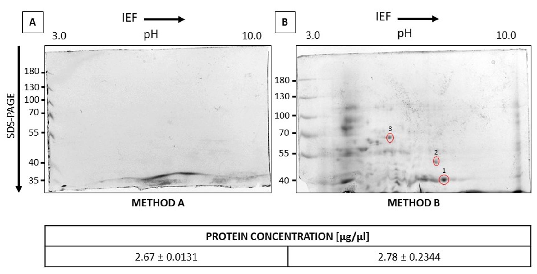
Figure 1. Optimization of the protein isolation method from L. luteus roots. 2-DE SDS-PAGE analysis for proteins isolated using the phenol (A) and modified Tris-EDTA (B) methods. For protein isolation, 1 g of roots was ground in a mortar with liquid nitrogen. Isoelectric focusing was performed according to the manufacturer’s instructions using the ReadyPrepTM 2-D Starter Kit. Electrophoretic separation was carried out at a constant voltage of 70 V for approximately 6 h. The gels were stained with Coomassie Brilliant Blue solution and then incubated in a destaining mixture of 20% (v/v) ethanol and 12% (v/v) acetic acid. The selected spots (marked as 1, 2, and 3) were identified.
Results of 2-DE SDS-PAGE analysis for proteins isolated using Methods I, II, III, and IV
The choice of solvent for TCA precipitation significantly affects protein recovery and sample quality (Figure 2). Acetone is commonly used with TCA to enhance protein denaturation, promote aggregation, and efficiently remove lipids and hydrophobic contaminants that may interfere with downstream proteomic analyses. It also dehydrates the sample, improving precipitation efficiency and reducing protein loss compared to TCA in water. This is evident in the lower protein concentrations observed in samples precipitated with TCA in water (Methods III and IV) compared to those treated with TCA in acetone (Methods I and II). Water-based precipitation is less effective, particularly for highly soluble or acid-sensitive proteins, resulting in reduced yield. These differences are reflected in the SDS-PAGE gel images. Methods III and IV result in fewer protein spots, poor separation, a cloudy background, and visible artifacts or contaminant bands, suggesting incomplete precipitation. In contrast, gels from Methods I and II (TCA in acetone) exhibit well-resolved, distinct protein spots of varying intensity, distributed across the gel, with a clear background and minimal artifacts. Prolonged precipitation (12 h) in method II negatively affects protein separation, causing co-migration and overlapping spots, and reducing the number of high-resolution, dense spots, despite the nearly twofold increase in protein concentration in the extracts. Moreover, prolonged precipitation using Methods II and IV leads to the loss of acidic pI spots, most likely as a result of time-dependent destabilization of the buffer system. Collectively, these findings demonstrate that 1-h precipitation with TCA in acetone offers superior efficiency, yielding cleaner protein extracts more suitable for high-resolution proteomic analyses.
Based on our optimization protocol, we present a schematic overview of the key steps and comparative methods for isolating and analyzing lupine root proteins by 2-DE (Figure 3). For details, see the text.
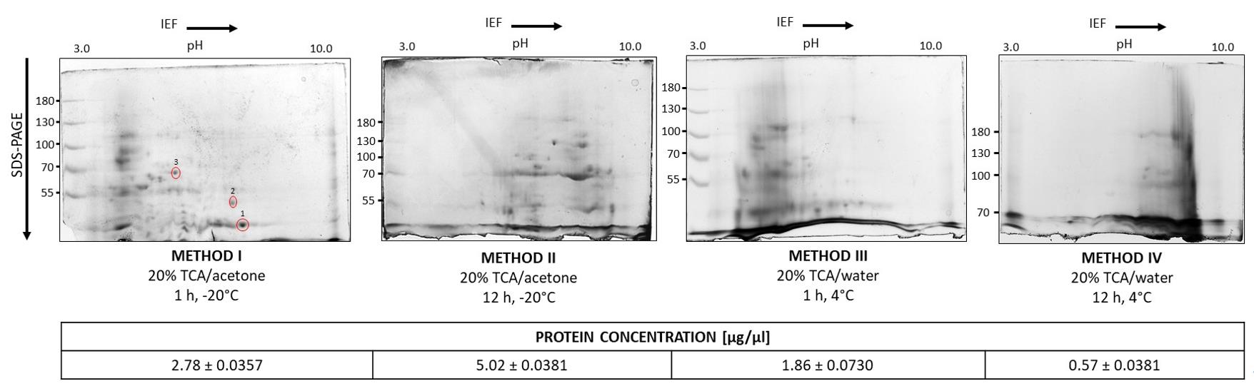
Figure 2. Optimization of the method for precipitation of proteins from lupine roots. To optimize the protein precipitation procedure, proteins from the extracts were precipitated using a 20% (w/v) TCA/acetone solution (Methods I and II) or a 20% (w/v) TCA/water solution (Methods III and IV). Two precipitation time variants were also tested: 1 h for Methods I and III, and 12 h for Methods II and IV. For isoelectric focusing, 120 μg of protein was applied. Isoelectric focusing was performed according to the manufacturer’s instructions (ReadyPrepTM 2-D Starter Kit). Electrophoretic separation was carried out at a constant voltage of 70 V for approximately 6 h. The gels were stained with Coomassie Brilliant Blue solution and then incubated in a destaining mixture of 20% (v/v) ethanol and 12% (v/v) acetic acid. The selected spots (marked as 1, 2, and 3) were identified.
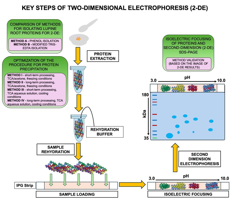
Figure 3. Workflow and comparative methods for two-dimensional electrophoresis (2-DE) of lupine root proteins
General notes and troubleshooting
General notes
1. While the current methodology has been validated for 2-DE proteomic profiling of lupine root tissues, interspecific variations in plant physiology, such as differential phenolic compound production and cell wall composition, necessitate species-specific optimization using our protocol for broader taxonomic applicability.
2. Improper root sampling procedures risk introducing nodule-derived proteins (e.g., nitrogenase complexes and bacteroid-specific markers) into plant tissue analyses. Cross-contamination arises when symbiotic root nodules are inadvertently included during root excision, compromising proteomic specificity.
3. A primary limitation of 2-DE lies in the physicochemical conflict between protein solubilization requirements and IEF parameters. Effective solubilization necessitates ionic detergents, which disrupt IEF’s fundamental requirement for electrically neutral conditions to maintain stable pH gradients.
Troubleshooting
Problem 1: Fragmentation or degradation of proteins.
Possible causes: Delayed sample heating or insufficient inhibition of endogenous proteases.
Solutions: Immediately heat samples after adding SDS-containing buffer to rapidly denaturate proteases. Include protease inhibitors (e.g., PMSF, EDTA) during cell lysis and keep samples on ice to minimize enzymatic activity.
Problem 2: Incomplete protein solubilization.
Possible causes: Inadequate concentration of chaotropic agents (e.g., urea/thiourea) or detergents in the lysis buffer/ interference from lipids, nucleic acids, or polysaccharides.
Solutions: For hydrophobic proteins, use a lysis buffer containing 7 M urea, 2 M thiourea, and 4% (w/v) CHAPS. Remove interfering substances by TCA/acetone precipitation. If necessary, extend incubation time and treat samples with RNase and DNase to degrade nucleic acids.
Problem 3: Horizontal streaking across the gel.
Possible causes: Incomplete protein solubilization or aggregation. If reduction and alkylation are insufficient, disulfide bonds can reform during focusing, leading to aggregation of basic proteins and horizontal streaks. Residual salts or ionic detergents further disrupt the pH gradient and impede uniform protein migration. It is necessary to disrupt disulfide-driven aggregation, remove interfering ions, and stabilize the pH gradient, thereby resolving horizontal streaking in the basic region.
Solution 1: After initial focusing, perform the reduction-alkylation step using ReadyPrep™ Reduction-Alkylation Kit (Bio-Rad Laboratories, Inc., Hercules, California, USA, catalog number: 163-2090) to irreversibly block thiols and prevent re-formation of disulfide bonds.
Solution 2: Decrease protein load by 20%–30% to avoid overloading artifacts.
Solution 3: Extend the IEF program to ensure proteins fully reach their pI.
Solution 4: Eliminate salts and ionic detergents by TCA/acetone precipitation with multiple acetone washes, thereby removing conductive contaminants and stabilizing the pH gradient.
Problem 4: Vertical streaking of protein spots.
Possible cause: Air bubbles trapped between the IPG strip and the second-dimension SDS-PAGE gel.
Solution: Degas molten agarose thoroughly before overlaying to ensure a bubble-free interface between the IPG strip and the gel.
Problem 5: Poor protein spot resolution (elongation or smearing).
Possible causes: Uneven SDS-PAGE gel polymerization/voltage instability during electrophoresis.
Solutions: Prepare gels with freshly made APS and TEMED, and degas acrylamide solutions before casting/maintaining a stable voltage (typically 100–150 V) during electrophoresis.
Problem 6: Weak or undetectable protein spots.
Possible causes: Protein loss during transfer from the IPG to the SDS gel/use of a detection method with low sensitivity (e.g., Coomassie staining for low-abundance proteins).
Solutions: Optimize equilibration conditions to improve protein transfer efficiency. For low-abundance proteins, use more sensitive detection methods, such as fluorescence-based stains or immunoblotting.
Acknowledgments
Conception and design of the study, A.K., E.W.; Investigation, S.B., P.W., E.W.; Data analysis and literature review, A.K., E.W.; Writing—original draft, S.B., A.K., E.W.; Evaluation of the final version of Ms: P.W., M.O.; Funding acquisition, S.B, E.W.; Supervision, E.W.
This research was funded by the Ministry of Science and Higher Education—funds for a research project awarded to S.B., supervised by E.W. (Diamond Grant IX program no. 0180/DIA/2020/49).
We are grateful to Professor Jaroslaw Tyburski (Department of Plant Physiology and Biotechnology, Nicolaus Copernicus University in Torun) for the opportunity to use the PROTEAN i12 IEF.
Competing interests
The authors declare no conflicts of interest.
References
- Jorrín Novo, J. V. (2015). Scientific standards and MIAPEs in plant proteomics research and publications. Front Plant Sci. 6: e00473. https://doi.org/10.3389/fpls.2015.00473
- Carpentier, S. C., Witters, E., Laukens, K., Deckers, P., Swennen, R. and Panis, B. (2005). Preparation of protein extracts from recalcitrant plant tissues: An evaluation of different methods for two‐dimensional gel electrophoresis analysis. Proteomics. 5(10): 2497–2507. https://doi.org/10.1002/pmic.200401222
- Isaacson, T., Damasceno, C. M. B., Saravanan, R. S., He, Y., Catalá, C., Saladié, M. and Rose, J. K. C. (2006). Sample extraction techniques for enhanced proteomic analysis of plant tissues. Nat Protoc. 1(2): 769–774. https://doi.org/10.1038/nprot.2006.102
- Wang, W., Vignani, R., Scali, M. and Cresti, M. (2006). A universal and rapid protocol for protein extraction from recalcitrant plant tissues for proteomic analysis. Electrophoresis. 27(13): 2782–2786. https://doi.org/10.1002/elps.200500722
- Chen, S. and Harmon, A. C. (2006). Advances in plant proteomics. Proteomics. 6(20): 5504–5516. https://doi.org/10.1002/pmic.200600143
- Niu, L., Zhang, H., Wu, Z., Wang, Y., Liu, H., Wu, X. and Wang, W. (2018). Modified TCA/acetone precipitation of plant proteins for proteomic analysis. PLoS One. 13(12): e0202238. https://doi.org/10.1371/journal.pone.0202238
- Damerval, C., De Vienne, D., Zivy, M. and Thiellement, H. (1986). Technical improvements in two‐dimensional electrophoresis increase the level of genetic variation detected in wheat‐seedling proteins. Electrophoresis. 7(1): 52–54. https://doi.org/10.1002/elps.1150070108
- Saravanan, R. S. and Rose, J. K. C. (2004). A critical evaluation of sample extraction techniques for enhanced proteomic analysis of recalcitrant plant tissues. Proteomics. 4(9): 2522–2532. https://doi.org/10.1002/pmic.200300789
- Fic, E., Kedracka‐Krok, S., Jankowska, U., Pirog, A. and Dziedzicka‐Wasylewska, M. (2010). Comparison of protein precipitation methods for various rat brain structures prior to proteomic analysis. Electrophoresis. 31(21): 3573–3579. https://doi.org/10.1002/elps.201000197
- Simpson, D. M. and Beynon, R. J. (2009). Acetone Precipitation of Proteins and the Modification of Peptides. J Proteome Res. 9(1): 444–450. https://doi.org/10.1021/pr900806x
- Alias, N., Mohd Aizat, W., Amin, N. D. M., Muhammad, N., Mohd Noor, N. (2017). A simple protein extraction method for proteomic analysis of mahogany (Swietenia macrophylla) embryos. Plant Omics. 10(4): 176–182. https://doi.org/10.1016/j.jprot.2009.01.011
- Balbuena, T. S., Silveira, V., Junqueira, M., Dias, L. L., Santa-Catarina, C., Shevchenko, A. and Floh, E. I. (2009). Changes in the 2-DE protein profile during zygotic embryogenesis in the Brazilian Pine (Araucaria angustifolia). J Proteomics. 72(3): 337–352. https://doi.org/10.1016/j.jprot.2009.01.011
- Orzoł, A. and Piotrowicz-Cieślak, A. I. (2017). Levofloxacin is phytotoxic and modifies the protein profile of lupin seedlings. Environ Sci Pollut Res. 24(28): 22226–22240. https://doi.org/10.1007/s11356-017-9845-0
- Frankowski, K., Wilmowicz, E., Kućko, A., Zienkiewicz, A., Zienkiewicz, K. and Kopcewicz, J. (2015). Molecular cloning of the BLADE-ON-PETIOLE gene and expression analyses during nodule development in Lupinus luteus. J Plant Physiol. 179: 35–39. https://doi.org/10.1016/j.jplph.2015.01.019
- Burchardt, S., Czernicka, M., Kućko, A., Pokora, W., Kapusta, M., Domagalski, K., Jasieniecka-Gazarkiewicz, K., Karwaszewski, J. and Wilmowicz, E. (2024). Exploring the response of yellow lupine (Lupinus luteus L.) root to drought mediated by pathways related to phytohormones, lipid, and redox homeostasis. BMC Plant Biol. 24(1): 1049. https://doi.org/10.1186/s12870-024-05748-4
- Nisar, M. and Hussain, H. (2020). The protein extraction method of Metroxylon sagu leaf for high-resolution two-dimensional gel electrophoresis and comparative proteomics. Chem Biol Technol Agric. 7(1): 14. https://doi.org/10.1186/s40538-020-00180-w
- Azri, W., Ennajah, A. and Jing, M. (2013). Comparative study of six methods of protein extraction for two-dimensional gel electrophoresis of proteomic profiling in poplar stems. Can J Plant Sci. 93(5): 895–901. https://doi.org/10.4141/cjps2013-113
- Bradford, M. M. (1976). A rapid and sensitive method for the quantitation of microgram quantities of protein utilizing the principle of protein-dye binding. Anal Biochem. 72: 248–254. https://doi.org/10.1016/0003-2697(76)90527-3
- Ogita, Z. I. and Markert, C. L. (1979). A miniaturized system for electrophoresis on polyacrylamide gels. Anal Biochem. 99(2): 233–241. https://doi.org/10.1016/s0003-2697(79)80001-9
Article Information
Publication history
Received: Jun 6, 2025
Accepted: Aug 26, 2025
Available online: Sep 9, 2025
Published: Oct 5, 2025
Copyright
© 2025 The Author(s); This is an open access article under the CC BY-NC license (https://creativecommons.org/licenses/by-nc/4.0/).
How to cite
Burchardt, S., Wojtaczka, P., Kućko, A., Ostrowski, M. and Wilmowicz, E. (2025). Advancing 2-DE Techniques: High-Efficiency Protein Extraction From Lupine Roots. Bio-protocol 15(19): e5461. DOI: 10.21769/BioProtoc.5461.
Category
Plant Science > Plant biochemistry > Protein > Isolation and purification
Systems Biology > Proteomics
Biochemistry > Protein > Electrophoresis
Do you have any questions about this protocol?
Post your question to gather feedback from the community. We will also invite the authors of this article to respond.