- Protocols

- Articles and Issues
- For Authors
- About
- Become a Reviewer

Fluorescence Lifetime-Based Separation of FAST-Labeled Cellular Compartment
Published: Vol 15, Iss 19, Oct 5, 2025 DOI: 10.21769/BioProtoc.5460 Views: 1347
Reviewed by: Aleksandra J. WierzbaAnonymous reviewer(s)
Original research article
The authors used this protocol in:

Jul 2024

Protocol Collections
Comprehensive collections of detailed, peer-reviewed protocols focusing on specific topics


Abstract
Here, we present a protocol for implementing the fluorogen-activating protein FAST (fluorescence-activating and absorption-shifting tag) in fluorescence lifetime imaging microscopy (FLIM), which allows separating fluorescent species in the same spectral channel based on fluorescence lifetime properties. Previous studies have demonstrated FLIM multiplexing using various combinations of synthetic probes, fluorescent proteins, or self-labeling tags. In this protocol, we utilize engineered FAST point mutation variants that bind fluorogen HBR-2,5-DM. The designed probes possess nearly identical, compact protein sizes (14 kDa), and the resulting protein–fluorogen complexes demonstrate comparable steady-state optical properties and exhibit distinct fluorescence lifetimes, displaying monoexponential fluorescence decay kinetics. When FAST variants are expressed with localization signals, these properties facilitate robust signal separation in regions with co-localized or spatially overlapping labels (nucleus and cytoskeleton in this protocol) in live mammalian cells. This method can be applied to separate other overlapping cellular compartments, such as the nucleus and Golgi apparatus, or mitochondria and cytoskeleton.
Key features
• The protocol employs FAST protein technology for fluorescent labeling.
• Separation of cellular compartments in the green channel (emission wavelength ~500–550 nm) using fluorescence lifetime data.
• Requires no coding skills.
• The protocol is optimized for SPCImage software.
Keywords: FLIMBackground
A high density of acquired information is often desired from a single sample, which requires the use of advanced multiplexed imaging systems. One way to achieve this is through the implementation of fluorescence lifetime measurements (FLIM). FLIM measures the fluorescence decay time of molecules. This technique allows for distinguishing spectrally similar probes as long as their excited states exist for significantly different durations before photon emission [1]. In time-correlated single photon counting (TCSPC) FLIM implementation, each pixel of an acquired image consists of a histogram of single photon counts per time bin. These lifetime histograms may be fitted with exponential decay functions. Parameters of the function (an, τn) can then be used for the separation of different fluorophores. Another approach for lifetime separation is the fit-free phasor approach, which uses a 2D representation to cluster pixels with similar lifetimes in phasor space.
Fluorogen-activating proteins are nonfluorescent proteins that can bind specific dyes called fluorogens [2]. Fluorogens in their free form are also nearly nonfluorescent molecules, but binding within protein pockets stabilizes their structure and results in increased fluorescence quantum yield. Fluorescence lifetimes may depend on the fluorophore's surrounding conditions [3,4], and due to this property, fluorogen-activating proteins have proven to be excellent tools in FLIM [5–7]. In this case, the microenvironment of fluorogens is essentially determined by the fluorogen-activating protein binding pocket. The FAST is one of the most extensively studied fluorogen-activating proteins [8,9]. This protein offers several advantages: it is significantly smaller than conventional fluorescent proteins (14 kDa) and requires neither time nor oxygen for maturation. By studying the 3D structure of FAST, we developed a set of point mutants with significant alterations in the characteristics of the resulting protein–fluorogen complexes [10]. Further investigation allowed us to select several FAST variants (R52K, P68T, P68K, and F62L) with similar brightness and dissociation constants of complexes with HBR-2,5-DM fluorogen and to apply them for fluorescence lifetime multiplexing in cellulo (in living cells). Here, we describe a detailed protocol for the separation of two cellular compartments (nucleus and cytoskeleton) using FLIM data.
This protocol is applicable for separating other overlapping compartments across different cell lines. Such applications may require optimization of transfection conditions to obtain compartments with comparable fluorescence signal intensities, which significantly facilitates successful data analysis. When selecting compartment pairs for study, the importance of achieving similar fluorescence intensities should be considered.
The Phasor approach described in data analysis enables separation of triplets of FAST variants; however, in this case, separation would rely on visual control of the expected compartment morphologies.
While other fluorogens can be used in combination with FAST in FLIM, they do not allow for the most successful data analysis approach (the fitting-based approach with fixed τ).
Materials and reagents
Biological materials
1. HeLa cell line (ATCC CCL-2)
Reagents
1. DMSO (Thermo Scientific Chemicals, catalog number: 327182500); store at 4 °C
2. DMEM (PanEco, catalog number: С410п); store at 4 °C
Note: Commercially available international equivalent: DMEM, high glucose (Gibco, catalog number: 11965092)
3. FAST variants constructs with localization signals [5,6]; please contact the corresponding author for constructs
Note: R52K, P68T, P68K, and F62L FAST variants can be used in the protocol. The separation of the vimentin-P68T and H2B-F62L pair is demonstrated as an example in the Data analysis section.
4. Fetal bovine serum (FBS) (Biosera, catalog number: FB-1001/500); store at -20 °C
5. Fluorogen HBR-2,5-DM [(Z)-5-(4-Hydroxy-2,5-dimethylbenzylidene)-2-thioxo-1,3-thiazolidin-4-one] [11]; please contact the corresponding author for fluorogen; store at -20 °C
6. Hanks’ balanced salt solution (HBSS) (PanEco, catalog number: Р020п); store at 4 °C
Note: Commercially available international equivalent: HBSS, calcium, magnesium, no phenol red (Gibco, catalog number: 14025092)
7. HEPES (Gibco, catalog number: 15630056); store at 4 °C
8. Opti-MEM powder (Gibco, catalog number: 22600134); store at 4 °C
9. Penicillin-Streptomycin, 100× solution (PanEco, catalog number: А063п'); store at -20 °C
Note: Commercially available international equivalent: Sigma-Aldrich, catalog number: P4333.
10. Polyethylenimine (PEI) (Polysciences, catalog number: 23966-1); store at -20 °C
11. Sodium bicarbonate (Thermo Scientific Chemicals, catalog number: 424270010); store at room temperature
12. Trypsin, powder (Gibco, catalog number: 27250018); store at 4 °C
13. Versene solution (PanEco, catalog number: Р080п); store at 4 °C
Note: Commercially available international equivalent: Gibco, catalog number: 15040066.
Solutions
1. DMEM complete (see Recipes)
2. HBR-2,5-DM stock solution (see Recipes)
3. HBR-2,5-DM-containing imaging solution (see Recipes)
4. Imaging media (see Recipes)
5. Opti-MEM (see Recipes)
6. Trypsin-Versene solution (see Recipes)
Recipes
1. DMEM complete
| Reagent | Final concentration | Quantity or volume |
|---|---|---|
| DMEM | n/a | 44.5 mL |
| FBS | 10% | 5 mL |
| Penicillin-streptomycin, 100× solution | 1× | 0.5 mL |
Note: Store at 4 °C for up to a month.
2. HBR-2,5-DM stock solution
| Reagent | Final concentration | Quantity or volume |
|---|---|---|
| HBR-2,5-DM | 10 mM | 5.34 mg |
| DMSO | n/a | 2 mL |
Note: Prepare 20 μL aliquots. Store at -20 °C for up to 3 months. Avoid repeated freeze-thaw cycles.
3. HBR-2,5-DM-containing imaging solution
| Reagent | Final concentration | Quantity or volume |
|---|---|---|
| HBR-2,5-DM stock solution | 5 μM | 10 μL |
| DMSO | n/a | 20 mL |
Note: Add the HBR-2,5-DM stock solution to the imaging solution and mix thoroughly by vigorous vortexing. Prepare the fluorogen-containing imaging solution fresh for each experiment, as storage beyond 24 h is not recommended due to potential degradation of the fluorogen.
4. Imaging solution
| Reagent | Final concentration | Quantity or volume |
|---|---|---|
| HBSS | n/a | 49.5 mL |
| HEPES 1 M | 10 mM | 0.5 mL |
Note: Store at 4 °C for up to 3 months.
5. Opti-MEM
| Reagent | Final concentration | Quantity or volume |
|---|---|---|
| Opti-MEM powder | 1.4% | 6.795 g |
| Sodium bicarbonate powder | 2.4 g/L | 1.2 g |
| Distilled water | n/a | 500 mL |
Note: Store at 4 °C for up to 3 months.
6. Trypsin-Versene solution
| Reagent | Final concentration | Quantity or volume |
|---|---|---|
| Versene solution | n/a | 50 mL |
| Trypsin powder | 0.25% | 125 mg |
Note: Store at 4 °C for up to a month.
Laboratory supplies
1. 10 μL filtered pipette tips (Vertex, catalog number: 4117NSF)
2. 10 mL serological pipette (Greiner CELLSTAR, catalog number: 607160)
3. 1,000 μL filtered pipette tips (Vertex, catalog number: 4337NSF)
4. 1.5 mL microtube (SSI Bio, catalog number: 1260-00)
5. 20 μL filtered pipette tips (Vertex, catalog number: 4237NAF)
6. 200 μL filtered pipette tips (Vertex, catalog number: 4237NSF)
7. 35 mm glass-bottomed culture dish (SPL Life Sciences, catalog number: 100350)
8. T25 culture flask (SPL Life Sciences, catalog number: 70025)
Equipment
1. 0.5–10 μL micropipette (Eppendorf, catalog number: 3123000020)
2. 100–1,000 μL micropipette (Eppendorf, catalog number: 3123000063)
3. 2–20 μL micropipette (Eppendorf, catalog number: 3123000039)
4. 20–200 μL micropipette (Eppendorf, catalog number: 3123000055)
5. Cell culture incubator (Sanyo, model: MCO-175)
6. FLIM equipment: Manual TE2000-U microscope (Nikon), confocal scanning system DCS-120 (Becker and Hickl), GVD - 120 galvo scanner control + GDA amplifier (Becker and Hickl) equipped with the 30/70 mirror as beamsplitter, 100× S Fluor 0.5–1.3 oil iris objective (Nikon); Laser WhiteLase SC480-6 (Fianium), AOTF module (Fianium), 480/10× filter (Chroma) (to cut residual “white” spectrum); TCSPC modules SPC-150 (Becker and Hickl), PMC-100-1 detectors (Becker and Hickl), HQ495LP, HQ525/50 (Chroma); Type F immersion oil (Leica, catalog number: 11513859)
Note: Alternative FLIM equipment configurations can be used for this protocol. If necessary, consult with a FLIM specialist.
7. Laminar flow cabinet (Labconco, model: MP-Logic Class II, Type A2 Biological Safety Cabinets)
8. Large capacity pipette (Hangzhou Miu Instruments, model: LEP-100)
9. Vortex Microspin FV-2400 (Biosan, catalog number: BS-010201-AAA)
10. Water bath thermostat (ELMI, model: TW-2.03)
Software and datasets
1. FIJI 1.53t (August 2022); free, open source
2. SPCImage software 8.9 (December 2023); commercial license required
3. SPCM Data Acquisition Software v.9.81 (2023); commercial license required
Procedure
A. Cell culture and transfection
1. Select pairs of H2B- and vimentin-fused FAST variants using Table 1 as a reference for fluorescence lifetimes.
Notes:
1. We performed successful separation of FAST variants with ≥0.3 ns fluorescence lifetime difference.
2. Vimentin and nuclear structures have distinguishable morphologies with spatial overlap, effectively demonstrating the method's capabilities. The protocol is not restricted to this specific pair. We successfully separated combinations of FAST variants with other localization signals available in-house, including Lifeact (actin-binding peptide), ensconsin (tubulin-binding protein), peroxisomal targeting signal, mitochondrial intermembrane space targeting signal, and β4Gal-T1 (Golgi apparatus).
Table 1. Fluorescence lifetimes of FAST-HBR-2,5-DM complexes measured in cellulo
| FAST variant | Fluorescence lifetime* |
|---|---|
| R52K | 1.4 ns |
| P68T | 1.7 ns |
| P68K | 1.9 ns |
| F62L | 2.2 ns |
*Data for FAST variants expressed as H2B fusion constructs.
Note: While this table provides reference fluorescence lifetimes for FAST variants, the cellular environment can affect these values. In our experience, fluorescence lifetimes of vimentin-FAST fusion constructs show similar values to the corresponding H2B-FAST data presented above. We recommend conducting separate measurements for each variant in its intended cellular localization to obtain accurate values for your specific conditions, especially when imaging alternative cellular compartments.
2. Grow HeLa cells in 5 mL of DMEM complete medium (see Recipes) in a T25 culture flask until cells reach 80%–90% confluency. Maintain cultures in a cell culture incubator at 37 °C with 5% CO2.
3. Warm DMEM complete medium and Trypsin-Versene solution (see Recipes) to 37 °C.
4. Aspirate DMEM complete medium from the flask using a 10 mL serological pipette and a large-capacity pipette. Add to the flask 1 mL of Trypsin-Versene solution using a 1 mL micropipette, gently rock the flask 3 times, and remove the solution with the same micropipette to eliminate FBS-containing DMEM residues. Add 1 mL of Trypsin-Versene solution and return the culture flask to the incubator for 3–5 min.
5. During cell incubation with Trypsin-Versene, fill 35 mm glass-bottomed culture dishes with 2 mL of DMEM complete medium.
Notes:
1. Prepare three dishes per FAST variant pair to ensure sufficient data reproducibility.
2. We strongly recommend acquiring data for each FAST variant individually in the intended cellular localization to obtain accurate lifetime values for your specific conditions, not only as pairs.
6. Resuspend the detached cells from step A4 using a 1 mL micropipette by pipetting up and down five times. Add 3 mL of DMEM complete medium to neutralize trypsin activity and resuspend cells again using a 10 mL serological pipette by pipetting up and down five times.
7. Reserve 0.5 mL of cell suspension in the T25 culture flask for subsequent passaging and add 4.5 mL of DMEM complete medium to it. Add 3 drops (160 μL) of cell suspension to each prepared 35 mm glass-bottomed culture dish from step A5. Gently agitate the flask and dishes 10 times using a lightning-shaped motion (zigzag: forward-left, right, forward-left, back-right to start). Return cells to the cell culture incubator.
8. Grow cells on 35 mm glass-bottomed culture dishes until reaching 60% confluency.
9. Warm Opti-MEM (see Recipes) to room temperature.
10. Aspirate DMEM complete medium from cell-containing 35 mm glass-bottomed culture dishes using a 10 mL serological pipette and a large-capacity pipette, wash cells once with 1 mL of Opti-MEM, and add 0.5 mL of Opti-MEM to each dish. Return to the cell culture incubator and incubate for 1 h.
Note: This incubation time includes PEI–DNA complex formation; therefore, initiate the following protocol steps 30 min after the medium change in step A10.
11. In a 1.5 mL microtube, mix 250 μL of room temperature Opti-MEM (1 mL micropipette) with 4.5 μL of room temperature PEI (2–20 μL micropipette) per dish. In a separate 1.5 mL microtube, mix 250 μL of room temperature Opti-MEM (1 mL micropipette) with 0.3 μg of H2B-FAST variant coding plasmid and 1.2 μg of vimentin-FAST variant coding plasmid (both dissolved in nuclease-free water, room temperature) using a 0.5–10 μL micropipette per dish. Incubate both mixtures at room temperature for 5 min.
Note: Solutions for 1–3 dishes can be prepared in a single 1.5 mL microtube by scaling up the volumes accordingly.
12. Add the entire volume of the DNA-containing Opti-MEM mixture to the PEI-containing Opti-MEM using a 1 mL micropipette and vortex for 3 s. Incubate the resulting solution at room temperature for 20 min.
13. Using a 1 mL micropipette, add the DNA–PEI mixture dropwise to cell-containing 35 mm glass-bottomed culture dishes. Gently agitate 10 times. Return cells to the incubator and incubate for 3.5 h.
14. Aspirate Opti-MEM from cell-containing 35 mm glass-bottomed culture dishes using a 1 mL micropipette and replace it with DMEM complete medium (37 °C) using a 10 mL serological pipette and a large-capacity pipette. Return cells to the incubator and incubate for 24–48 h.
Notes:
1. FAST proteins do not require maturation time and can be imaged the following day. The experiment can be postponed for an additional day for convenience; however, avoid allowing cells to become overgrown.
2. Cells may be fixed with 4% paraformaldehyde (PFA) if required. We found no significant impact on fluorescence lifetimes for the H2B- and vimentin-FAST variant fusion constructs when using fixed samples. It should be noted that our testing was limited to this particular combination.
B. Live-cell fluorescence lifetime imaging microscopy
1. Prepare HBR-2,5-DM-containing imaging solution (see Recipes) on the day of the imaging experiment.
2. Aspirate DMEM complete medium from cell-containing dishes using a 10 mL serological pipette and a large-capacity pipette. Add 1 mL of room temperature imaging solution (see Recipes) using a 1 mL micropipette, gently rock the dishes three times, and remove the solution with the same micropipette to eliminate DMEM residues. Then, add 2 mL of room temperature HBR-2,5-DM-containing imaging solution using a 10 mL serological pipette and a large-capacity pipette. Incubate at room temperature for 5 min.
Note: HBR-2,5-DM-containing imaging solution utilizes pH buffering independent of the CO2/HCO3− system. Therefore, cell-containing dishes should be maintained outside the CO2 incubator environment.
3. Set the climate control system temperature at 25 °C and adjust the temperature of the room to avoid thermal shifts of equipment. Switch on the FLIM equipment.
Note: Avoid door openings and air winds near the microscope.
4. Add Type F immersion oil to the objective and put the sample into the holder.
5. Focus on the object using the eyepieces and switch the microscope to the confocal port.
Note: Check the sample fixation and focusing knob tension to ensure that the drift is appropriate during image acquisition.
6. Open SPCM software.
Note: There are basic steps of image acquisition. Please read the original Becker and Hickl Manual before starting.
7. In the Galvano Scanner menu (Devices → Galvano Scanner), push Preview and move the sample to find the appropriate field of view.
Note: The 100× objective with 1.3NA has aberration of the field. You can use a 2× or higher zoom of the selected field to obtain an image with uniform intensity distribution.
8. Adjust laser power and scan time.
Note: The analysis needs at least 103 photons per analysis point (individual pixel or several binned pixels, see step A2 of Data analysis). Time-correlated single photon counting (TCSPC) count rate has restrictions and must be lower than 1% of the laser repetition rate. In our setup, it was not higher than 6 × 10⁵ photons per second in the brightest pixel of the acquisition region (monitored via the left-bottom area of the software interface showing the ADC level).
9. Set StopT flag.
10. Set Repeat to frame in Galvano scanner control and scan 1 frame. Check the photon quantity (event number in the status bar, blue line in Device state area) and calculate the appropriate number of frames to obtain nearly 108 photons per final image. You can also set Repeat to continuous and set the appropriate Collection time.
Note: Set a higher number of frames. You can stop scanning earlier.
11. Push Start Scan to start acquisition.
12. After data collection is stopped, save the raw data as an .sdt file (Main → Save).
13. Export data to SPCImage (press F9) and save file as an .img file (Main → Save).
Data analysis
Note: We present three data analysis approaches. The first (Section A below, the τ-value approach) and third (Section C below, the fitting-based approach with fixed τ) methods employ fit-based algorithms that demand high computational resources. In contrast, the second (Section B below, the phasor approach) method is fit-free and can therefore be implemented on computers with limited processing power. However, the second approach has the limitation that phasor space clusters are determined visually rather than through rigorous numerical criteria. The third approach is our preferred method as it allows precise separation of overlapping compartments using strict numerical parameters. This approach is uniquely enabled by the HBR-2,5-DM fluorogen, which exhibits monoexponential fluorescence decay when paired with FAST variants. Figure 1 shows the final result of cellular compartment separation achieved using these methods.
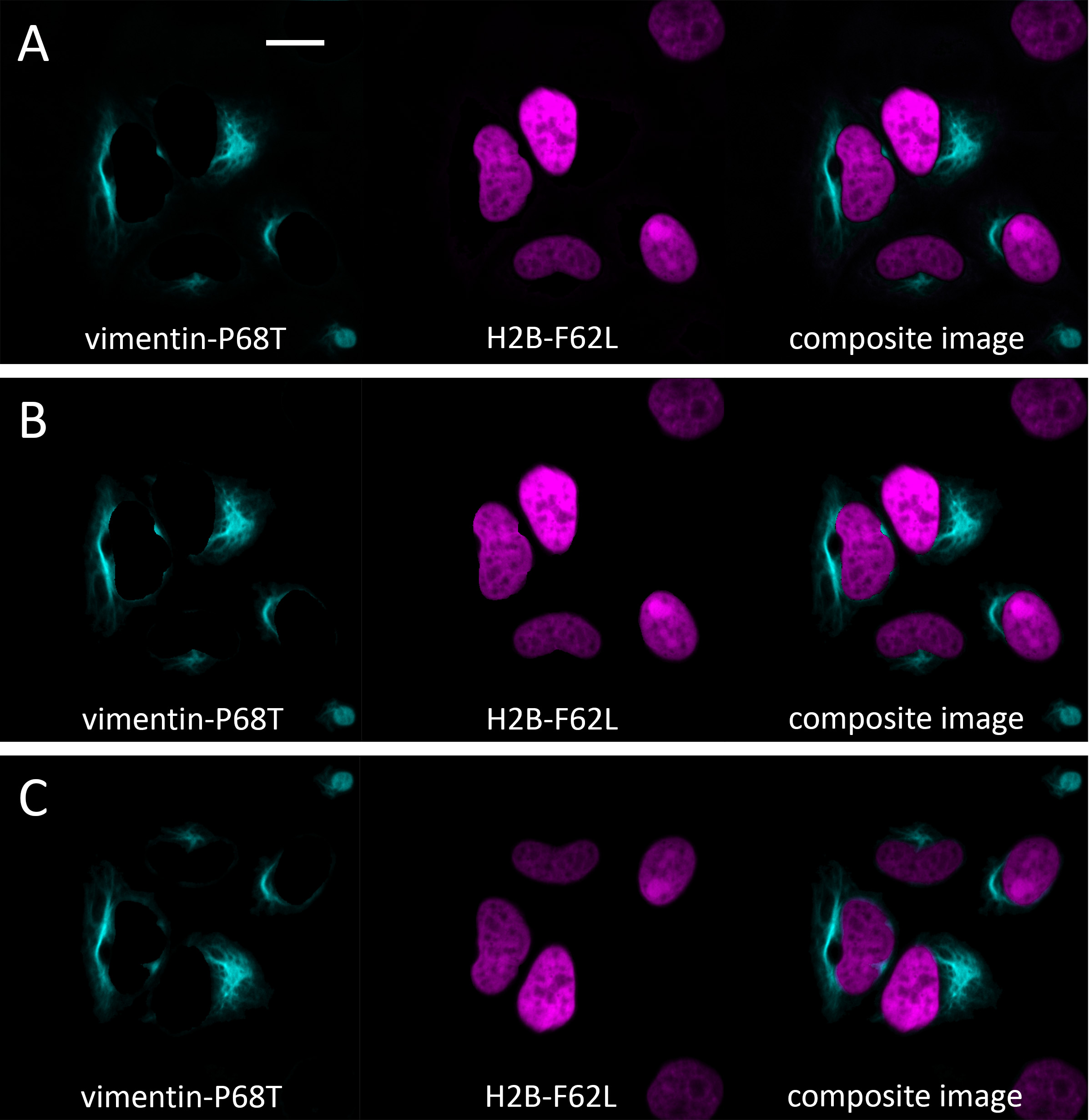
Figure 1. Final images acquired with (A) τ value approach, (B) phasor approach, and (C) fitting-based approach with fixed τ. The initial lifetime-coded color image is shown in Figure 2, left panel. Note that images acquired with a fitting-based approach with fixed τ are mirrored relative to the original image due to the matrix export format; this is the expected result from the analysis. This can be easily fixed in FIJI. Scale bar = 20 μm.
A. The τ-value approach
1. Position the blue crosshair in a visually uniform region of medium intensity within the cell (Figure 2, left panel).
Note: Intensity refers to photon count as indicated by the peak height in the decay graph (Figure 2, bottom-right panel).
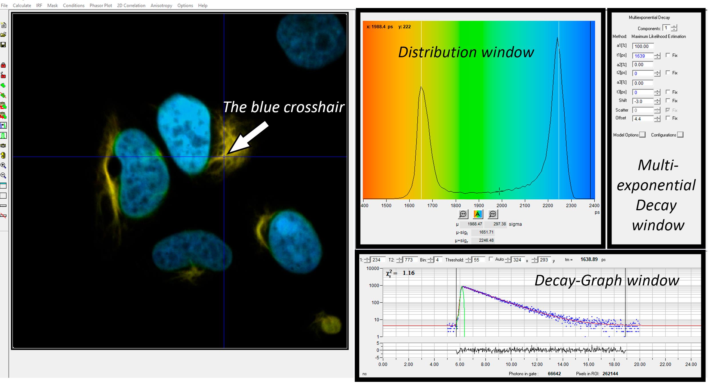
Figure 2. Screenshot of the SPCImage software. Black boxes mark parts of the interface with the names used in the protocol. White arrow indicates the blue crosshair showing which pixel's data is currently displayed and analyzed.
2. Set the binning factor such that the peak of the fluorescence lifetime curve reaches approximately 1,000 photons (Decay-Graph window, Figure 3A).
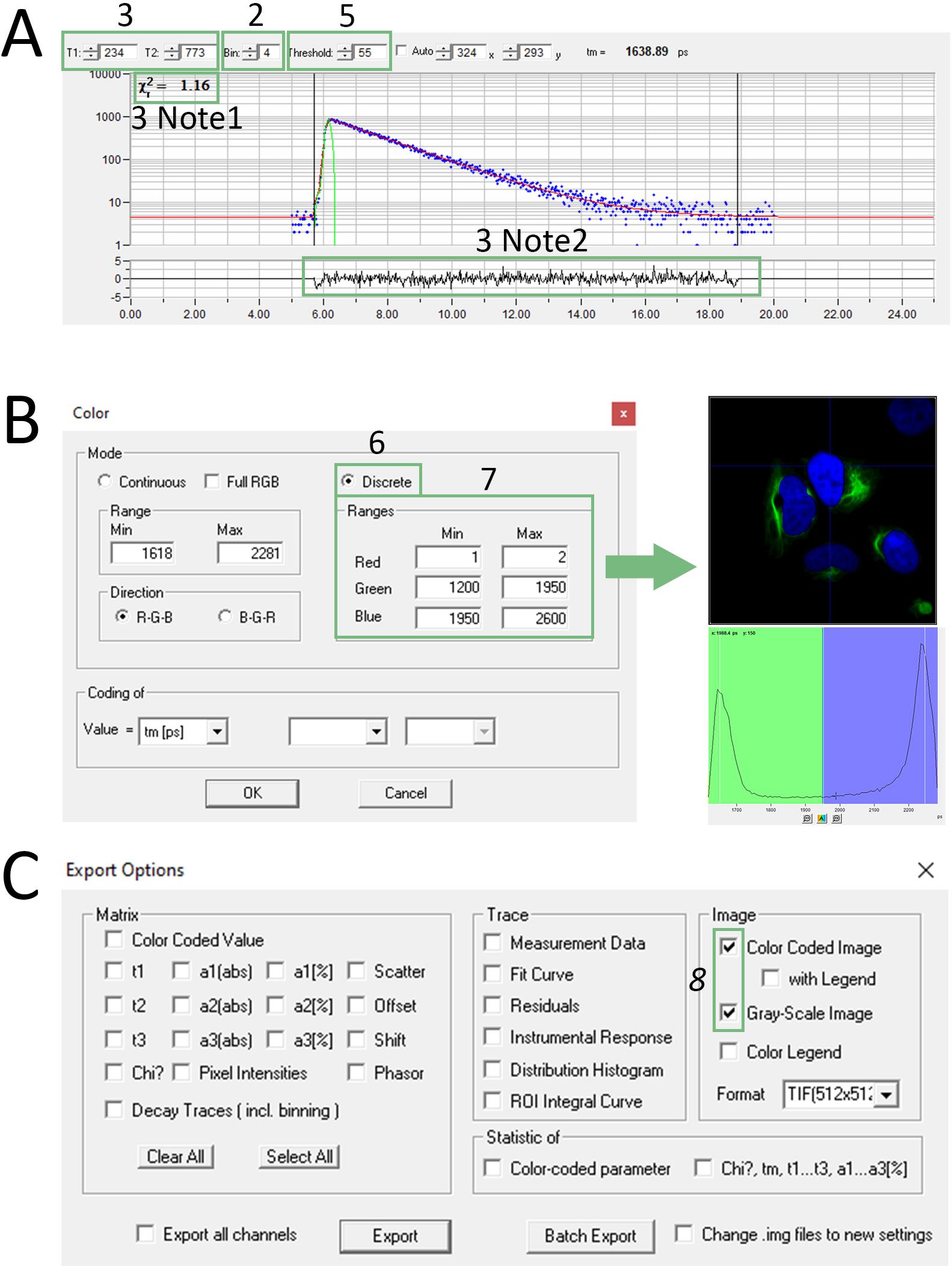
Figure 3. Screenshot of the SPCImage software for two cellular compartments separation with the τ-value approach. (A) Screenshot of Decay-Graph window; the numbers refer to steps A2, A3, and A5 and Notes 1, 2 in step A3. (B) Screenshot of Color window; the numbers refer to steps A6 and A7. The green arrow points to the screenshot of the resulting image after performing step A7. (C) Screenshot of Export Options window; the number refers to step A8.
3. Adjust T1 and T2 values to include the entire decay curve while excluding baseline regions (Decay-Graph window, Figure 3A).
Notes:
1. The Decay-Graph window displays the chi-squared value. A chi-square value ≤1.2 indicates an excellent fit. For values above 1.2, see Troubleshooting.
2. Examine residuals displayed beneath the fluorescence lifetime curve. In the case of a perfect fit, this line would be stochastic.
4. Generate the decay matrix (Calculate → Decay matrix in the main menu).
5. Adjust the threshold parameter in the Decay-Graph window to 50–150 to remove background pixels with low photon counts (Figure 3A). Generate a new decay matrix (Calculate → Decay matrix in the main menu).
6. Set color-coding to discrete mode (Options → Color in main menu, Mode discrete, Figure 3B).
7. Assign τ value ranges to each separate color channel. Choose ranges that include one photon peak in the histogram (displayed in the Distribution window, Figure 3B) corresponding to each FAST variant lifetime.
Note: When using two FAST variants, one channel will remain empty. Assign a narrow range (for example, from 1 to 2) to this channel (here, channel Red, Figure 3B).
8. Export resulting FLIM images (File → Export… in the main menu). Select both Color Coded Image and Grayscale Image boxes in Export options (Figure 3C).
Note: The Grayscale Image represents a total intensity image of the cells.
9. Import images into FIJI.
10. Transform colored images to RGB stack (Image → Type → RGB stack).
11. Separate images from stack (Image → Stacks → Stack to Images). Close the empty image.
12. Apply colorblind-friendly color coding to images (Image → LUT).
13. Merge channels to generate composite image (Image → Color → Merge Channels…).
B. The phasor approach
1. Repeat steps A1–5 from Data analysis. Check the chi-square values and residuals (see notes 1 and 2 in step A3 of A).
2. Calculate the phasor plot (Phasor plot button in the main menu).
3. Turn off the grayscale image overlay (Options → Preferences in the main menu, uncheck Grayscale Image overlay box, Figure 4A).
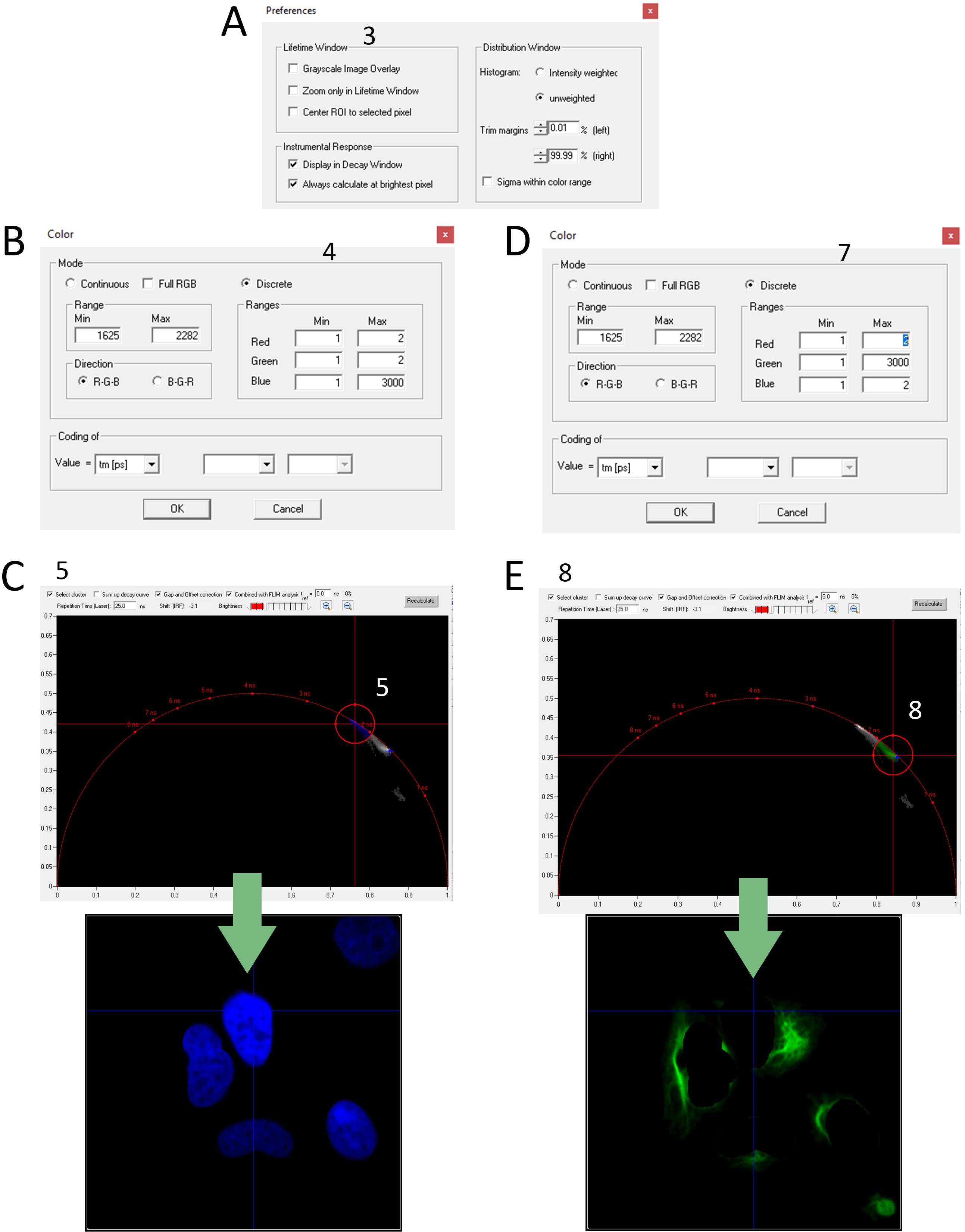
Figure 4. Screenshot of the SPCImage software for two cellular compartment separation with the phasor approach. (A) Screenshot of Preferences window; the number refers to step B3. (B) Screenshot of Color window; the number refers to step B4. (C). Screenshot of Phasor plot window; the number refers to step B5. The green arrow points to the screenshot of the resulting image after performing step B5. (D) Screenshot of Color window; the number refers to step B7. (E) Screenshot of Phasor plot window; the number refers to step B8. The green arrow points to the screenshot of the resulting image after performing step B8.
4. Set color-coding to discrete mode (Options → Color in the main menu, Mode discrete) and set the blue color range from 1 to 3,000 ps so that all τ values are colored blue. Set red and green channel ranges from 1 to 2 (Figure 4B).
5. Check the Select cluster box and select the first cluster (a group of pixels with similar fluorescence lifetime values on phasor space) (Figure 4C).
Note: Shape clusters based on expected FAST variant fluorescence lifetime.
6. Export the resulting FLIM image (File → Export… in the main menu). Select both Color Coded Image and Grayscale Image boxes in the export options.
Note: The Grayscale Image represents a total intensity image of the cells.
7. Set color-coding to discrete mode (Options → Color in the main menu, Mode discrete) and set the green color range from 1 to 3,000 ps so that all τ values are colored green. Set red and blue channel ranges from 1 to 2 (Figure 4D).
8. Select the second cluster (a group of pixels with similar fluorescence lifetime values on phasor space) (Figure 4E).
Note: Shape clusters based on expected FAST variant fluorescence lifetime.
9. Export the resulting FLIM image (File → Export… in the main menu). Select the Color Coded Image box in the export options.
10. Repeat steps A9–13 from Data analysis.
C. The fitting-based approach with fixed τ
1. Repeat steps A1–5 from Data analysis. Check the chi-square values and residuals (see notes 1 and 2 in step A3).
Note: Examination of chi-square values and residuals serves as quality control for photon collection and fitting procedures, ensuring reliable data even though these metrics are not used in downstream analysis.
2. Increase the number of exponential components to two in the Multiexponential Decay window (Figure 5A).
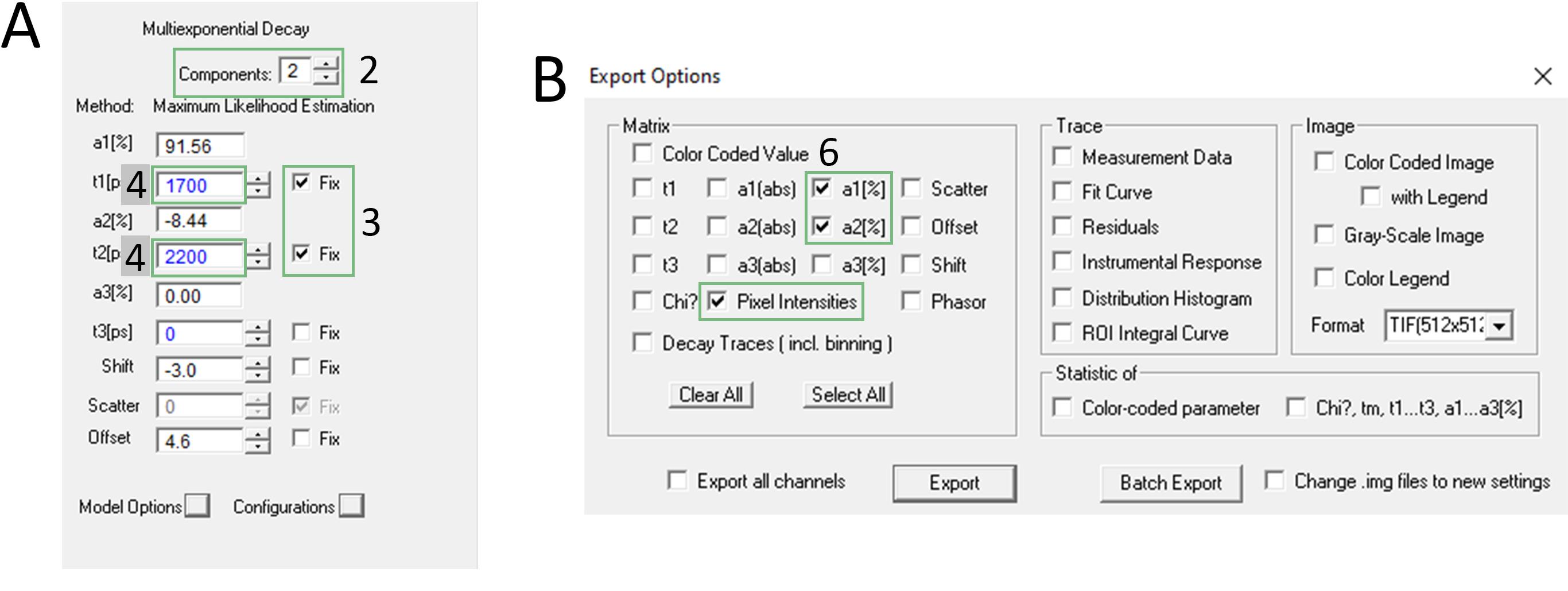
Figure 5. Screenshot of the SPCImage software for two cellular compartment separation with the fitting-based approach with fixed τ. (A) Screenshot of Multiexponential Decay window; the numbers refer to steps C2, C3, and C4. (B) Screenshot of Export Options window, the number refers to step C6.
3. Check the Fix box for both t1 and t2 components in the Multiexponential Decay window (Figure 5A).
4. Set t1 and t2 values in the Multiexponential Decay window to the expected values of the FAST variants used (Figure 5A).
5. Generate the decay matrix (Calculate → Decay matrix in the main menu).
6. Export matrices of a1(%) and a2(%) components and pixel intensities (File → Export… in the main menu, Figure 5B).
Note: Matrices will be mirrored relative to the original image; therefore, the Grayscale Image cannot be used in this case.
7. Import all matrices into FIJI (File → Import → Text Image…).
8. Convert all pixels with values <0.1% in a1[%] and a2[%] images to not-a-number (NaN) (Image → Adjust → Threshold…).
Note: Depending on the quality of the fit, the threshold value may need to be increased.
9. Multiply the pixel intensity image by a1[%] or a2[%] images (Process → Image Calculator…).
10. Apply colorblind-friendly color coding to images (Image → LUT).
11. Merge channels to generate composite image (Image → Color → Merge Channels…).
Validation of protocol
This protocol or parts of it has been used and validated in the following research article:
• Bogdanova et al. [5]. Fluorescence lifetime multiplexing with fluorogen activating protein FAST variants. Communications Biology (Figures 4–7).
General notes and troubleshooting
General notes
1. Other fluorogens can be used with FAST variants in fluorescence lifetime multiplexing (see [5] or [6]); however, in our experience, the fitting-based approach with fixed τ values worked optimally with HBR-2,5-DM only.
2. The fluorogens HBR-2,5-DM and HMBR are available for purchase from The Twinkle Factory (https://www.the-twinkle-factory.com/). Fluorogens are also available upon request from the corresponding author or can be synthesized in-house.
3. We strongly recommend acquiring data for each FAST variant lifetime at individual localizations separately before performing imaging of multiple FAST variants within a single cell.
4. Separation of mixed lifetimes using linear addition/combination in phasor space is a powerful approach; however, this function is not available in the SPCImage software. Software packages that support this feature will provide improved signal unmixing in phasor-based analysis.
5. Cells can be fixed prior to imaging using 4% PFA solution without significant alterations in fluorescence lifetimes.
6. The transfection procedure can be effectively carried out with alternative transfection reagents such as Lipofectamine LTX (Invitrogen, catalog number: 15338100) or FuGENE HD (Promega, catalog number: E2311).
Troubleshooting
Problem 1: Low photon count.
Possible cause: Low signal intensity.
Solution: Increase laser power or photon collecting time, optimize the optical configuration of your microscope, or optimize transfection efficiency.
Problem 2: High chi-square value and non-stochastic residuals.
Possible cause: Bad fitting.
Solution: Inspect the raw decay curve for obvious artifacts. Validate instrument response function (IRF) quality and re-measure it if necessary. Adjust T1 and T2 values. Test alternative decay models: increase the number of exponential components to two or three.
Acknowledgments
Conceptualization, M.B., Y.B.; Investigation, Y.B., I.S.; Writing—Original Draft, Y.B., I.S.; Writing—Review & Editing, A.S., M.B.; Funding acquisition, M.B.; Supervision, M.B. A.G., M.B., and Y.B. acknowledge the Ministry of Health of the Russian Federation (Assignment #124020900020-4). The protocol described here is based on research previously published in Bogdanova et al. [5].
Competing interests
The authors declare that they have no financial or non-financial competing interests.
References
- Datta, R., Heaster, T. M., Sharick, J. T., Gillette, A. A. and Skala, M. C. (2020). Fluorescence lifetime imaging microscopy: fundamentals and advances in instrumentation, analysis, and applications. J Biomed Opt. 25(7): 1–43. https://doi.org/10.1117/1.JBO.25.7.071203
- Hori, Y., Ueno, H., Mizukami, S. and Kikuchi, K. (2009). Photoactive yellow protein-based protein labeling system with turn-on fluorescence intensity. J Am Chem Soc. 131(46): 16610–16611. https://doi.org/10.1021/ja904800k
- Okabe, K., Inada, N., Gota, C., Harada, Y., Funatsu, T. and Uchiyama, S. (2012). Intracellular temperature mapping with a fluorescent polymeric thermometer and fluorescence lifetime imaging microscopy. Nat Commun. 3(1): 705. https://doi.org/10.1038/ncomms1714
- Suhling, K., Yahioglu, G., Le Marois, A., Hirvonen, L. M., Nedbal, J., Levitt, J. A., Chung, P.-H., Dreiss, C., Beavil, A., Beavil, R., et al. (2019). Fluorescence lifetime imaging for viscosity and diffusion measurements. In Periasamy, A. So, P. T. and König, K. (Eds.). Multiphoton Microscopy in the Biomedical Sciences XIX. SPIE. https://doi.org/10.1117/12.2508744
- Bogdanova, Y. A., Solovyev, I. D., Baleeva, N. S., Myasnyanko, I. N., Gorshkova, A. A., Gorbachev, D. A., Gilvanov, A. R., Goncharuk, S. A., Goncharuk, M. V., Mineev, K. S., et al. (2024). Fluorescence lifetime multiplexing with fluorogen activating protein FAST variants. Commun Biol. 7(1): 799. https://doi.org/10.1038/s42003-024-06501-1
- Gilvanov, A. R., Myasnyanko, I. N., Goncharuk, S. A., Goncharuk, M. V., Kublitski, V. S., Bodunova, D. V., Sidorenko, S. V., Maksimov, E. G., Baranov, M. S. and Bogdanova, Y. A. (2025). Fluorescence lifetime multiplexing with fluorogen-activating FAST protein variants and red-shifted arylidene-imidazolone derivative as fluorogen. Biosensors (Basel). 15(5). https://doi.org/10.3390/bios15050274
- El Hajji, L., Lam, F., Avtodeeva, M., Benaissa, H., Rampon, C., Volovitch, M., Vriz, S. and Gautier, A. (2024). Multiplexed in vivo imaging with fluorescence lifetime-modulating tags. Adv Sci. (Weinh.) 11(32): e2404354. https://doi.org/10.1002/advs.202404354
- Plamont, M.-A., Billon-Denis, E., Maurin, S., Gauron, C., Pimenta, F. M., Specht, C. G., Shi, J., Quérard, J., Pan, B., Rossignol, J., et al. (2016). Small fluorescence-activating and absorption-shifting tag for tunable protein imaging in vivo. Proc Natl Acad Sci USA. 113(3): 497–502. https://doi.org/10.1073/pnas.1513094113
- Mineev, K. S., Goncharuk, S. A., Goncharuk, M. V., Povarova, N. V., Sokolov, A. I., Baleeva, N. S., Smirnov, A. Y., Myasnyanko, I. N., Ruchkin, D. A., Bukhdruker, S., et al. (2021). NanoFAST: structure-based design of a small fluorogen-activating protein with only 98 amino acids. Chem Sci. 12(19): 6719–6725. https://doi.org/10.1039/d1sc01454d
- Goncharuk, M. V., Baleeva, N. S., Nolde, D. E., Gavrikov, A. S., Mishin, A. V., Mishin, A. S., Sosorev, A. Y., Arseniev, A. S., Goncharuk, S. A., Borshchevskiy, V. I., et al. (2022). Structure-based rational design of an enhanced fluorogen-activating protein for fluorogens based on GFP chromophore. Commun Biol. 5(1), 706. https://doi.org/10.1038/s42003-022-03662-9
- Li, C., Plamont, M.-A., Sladitschek, H. L., Rodrigues, V., Aujard, I., Neveu, P., Le Saux, T., Jullien, L. and Gautier, A. (2017). Dynamic multicolor protein labeling in living cells. Chem Sci. 8(8): 5598–5605. https://doi.org/10.1039/c7sc01364g
Article Information
Publication history
Received: Jun 26, 2025
Accepted: Aug 21, 2025
Available online: Sep 15, 2025
Published: Oct 5, 2025
Copyright
© 2025 The Author(s); This is an open access article under the CC BY-NC license (https://creativecommons.org/licenses/by-nc/4.0/).
How to cite
Gilvanov, A. R., Solovyev, I. D., Savitsky, A. P., Baranov, M. S. and Bogdanova, Y. A. (2025). Fluorescence Lifetime-Based Separation of FAST-Labeled Cellular Compartment. Bio-protocol 15(19): e5460. DOI: 10.21769/BioProtoc.5460.
Category
Cell Biology > Cell imaging > Fluorescence
Biophysics > Biophotonics
Do you have any questions about this protocol?
Post your question to gather feedback from the community. We will also invite the authors of this article to respond.