- Protocols

- Articles and Issues
- For Authors
- About
- Become a Reviewer

Analyzing RNA Localization Using the RNA Proximity Labeling Method OINC-seq
Published: Vol 15, Iss 15, Aug 5, 2025 DOI: 10.21769/BioProtoc.5403 Views: 2371
Reviewed by: Alessandro DidonnaAnonymous reviewer(s)
Original research article
The authors used this protocol in:
Mar 2025

Protocol Collections
Comprehensive collections of detailed, peer-reviewed protocols focusing on specific topics


Abstract
Thousands of RNAs are localized to specific subcellular locations, and these localization patterns are often required for optimal cell function. However, the sequences within RNAs that direct their transport are unknown for almost all localized transcripts. Similarly, the RNA content of most subcellular locations remains unknown. To facilitate the study of subcellular transcriptomes, we developed the RNA proximity labeling method OINC-seq. OINC-seq utilizes photoactivatable, spatially restricted RNA oxidation to specifically label RNA in proximity to a subcellularly localized bait protein. After labeling, these oxidative RNA marks are then read out via high-throughput sequencing due to their ability to induce predictable misincorporation events by reverse transcriptase. These induced mutations are then quantitatively assessed for each gene using our software package PIGPEN. The observed mutation rate for a given RNA species is therefore related to its proximity to the localized bait protein. This protocol describes procedures for assaying RNA localization via OINC-seq experiments as well as computational procedures for analyzing the resulting data using PIGPEN.
Key features
• OINC-seq assays the RNA content of a variety of subcellular locations.
• OINC-seq utilizes a photoactivatable, proximity-dependent RNA oxidation reaction to label RNAs.
• Oxidative RNA marks are read using high-throughput sequencing without the need for enrichment.
• Oxidative RNA marks are identified and quantified using the associated PIGPEN software.
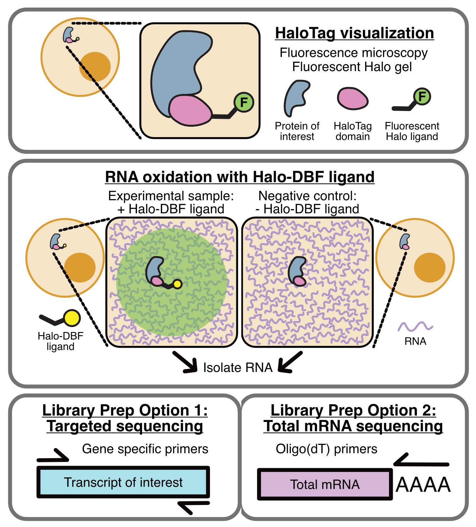
Keywords: Proximity labelingGraphical overview
Background
In a variety of organismal and developmental contexts, the localization of specific RNAs to specific subcellular locations promotes cellular and organismal function. For example, mate type switching in yeast [1] and developmental patterning in Drosophila [2,3] are controlled in part through the trafficking of specific mRNAs to precise subcellular locations. Mutations in RNA-binding proteins involved in RNA transport are associated with a variety of human neurological diseases [4,5]. However, for most localized RNAs, the mechanisms that govern their transport remain unknown. This includes the cis-elements within transcripts that mark them as RNAs to be localized, as well as the RNA-binding proteins (RBPs) that mediate the process.
A common experimental technique in the study of RNA localization is the characterization of RNA populations at subcellular locations. Historically, this has often been achieved through cellular fractionation, either by biochemical or mechanical means, followed by RNA isolation and characterization from the resulting fractions [6–12]. Although these techniques have led to many insights, they also have disadvantages. Mechanical cellular fractionations often require that the interrogated cell type have specific morphologies. For example, neurons are commonly separated into soma and neurite fractions, but the technique for doing so relies on cells having long, thin projections [7]. Biochemical fractionations, although more flexible regarding cell shape and morphology, have their own challenges. The association between an RNA and a subcellular location or organelle may be weak or transient and therefore lost during purification, leading to false negatives. Similarly, RNA molecules in subcellular environments that are spatially distinct within intact cells may nevertheless have similar biochemical properties and therefore copurify, leading to false positives.
Newer techniques that rely on proximity labeling remove many of these concerns. In these approaches, bait proteins are first localized to the subcellular location of interest [13–16]. Upon a chemical or light-based stimulus, RNAs in close proximity to the bait protein (usually 20–100 nm) are specifically labeled. In the majority of the techniques reported to date, these labels result in the biotinylation of bait-proximal RNAs, facilitating their downstream isolation with streptavidin and characterization.
OINC-seq builds on one of these RNA proximity labeling methods, Halo-seq [13,17]. In Halo-seq, a HaloTag-fused protein is specifically localized to the subcellular location of interest [18]. HaloTag domains covalently bind to Halo ligands. Upon addition of Halo-DBF ligand, a dibromofluorescein (DBF) molecule therefore assumes the same subcellular distribution as the Halo-tagged bait protein. When irradiated with green light, DBF emits singlet oxygen radicals that oxidize nearby RNAs. Because guanosine residues have the lowest redox potential of any of the four bases, they are preferentially oxidized to form 8-oxoguanosine as well as further oxidized hydantoins.
In Halo-seq, these oxidized guanosine residues are then alkynylated, which makes them substrates for biotinylation through Click chemistry. With OINC-seq, however, we sought to streamline the process to detect oxidized guanosines directly without the need for alkynylation, biotinylation, and purification. Instead, following the light-induced oxidation of bait-proximal RNA, total RNA is isolated and reverse transcribed. Reverse transcriptase predictably misinterprets oxidized guanosine [19], leading to G to T, G to C, and G deletion mutations in the resulting cDNA. Quantification of these mutations via high-throughput sequencing therefore provides a readout of the relative proximity of each RNA species to the Halo-tagged bait protein. In order to identify and quantify these mutations in RNAseq data, we developed the PIGPEN software. PIGPEN takes in RNAseq reads from an OINC-seq experiment and returns tables of mutation rates for each gene detected in the sample.
In general, OINC-seq experiments can take one of two forms. They can either be designed to assay the entire transcriptome, or they can be focused on one RNA through the interrogation of an amplicon. Although limited in focus to one RNA species, amplicon-based experiments typically have extensive read depth for the RNA of interest, leading to more accurate results. In contrast, although transcriptome-wide experiments interrogate thousands of RNA species at once, the reduced read depth assigned to any one RNA species can lead to noisier results.
Oxidation-induced mutations are relatively rare. This rarity requires that other, non-oxidation-derived sources of mutations be suppressed as much as possible. For example, Illumina sequencers miscall approximately 1 out of 1,000 bases in a typical sequencing reaction. In principle, it is impossible to distinguish between such a miscall and an oxidation-induced mutation. The usage of paired-end reads can mitigate this by requiring that any given mutation be seen in both reads of a mate pair in order to be classified as a true mutation and not a product of sequencer error. Specific options in PIGPEN implement this functionality.
RNA in close proximity to the bait protein may be expected to have multiple oxidation events and, therefore, multiple mutations along the same molecule. Random mutations, on the other hand, may be expected to be more evenly distributed across the entire RNA population. The appearance of multiple mutations within the same read might then give additional confidence in the localization of an RNA. Options in PIGPEN also support this functionality.
Finally, because of the rarity of oxidation-induced mutations, the fidelity of the polymerases used in the making of RNAseq libraries also matters. During the development of OINC-seq, we tested multiple library preparation kits and found that Quantseq kits from Lexogen consistently had the lowest background mutation rate in untreated samples, making them ideal for use with OINC-seq. However, these kits only interrogate the 3’ ends of molecules with poly-A tails. RNAs without these tails are therefore not assayable using this kit. It is possible that other library preparation methods would have suitable rates of background mutations, but they have not yet been tested. Amplicon-based experiments afford more flexibility in polymerase choice. We have found that the use of SuperScript IV for reverse transcription and NEB Q5 polymerase for PCR consistently leads to acceptably low levels of background mutations.
Materials and reagents
Biological materials
1. Cell line expressing HaloTag fusion protein
Note: In this protocol, authors use HeLa cells (ATCC, catalog number: CCL-2).
Reagents
1. Cell culture medium specific to the cell line used. In this protocol, the authors used the following formulation for HeLa cell culture: DMEM + D-Glucose + L-Glutamine (Gibco, catalog number: 11965-092), 10% EqualFETAL serum (Atlas Biologicals, catalog number: EF-0500-A), and 1% penicillin-streptomycin (Gibco, catalog number: 15140-122)
2. Doxycycline hydrochloride (Fisher Scientific, catalog number: AAJ6042203v)
3. Phosphate-buffered saline (PBS) (Invitrogen, catalog number: AM9625)
4. Hank’s balanced salt solution (HBSS) without calcium or phenol red (VWR, catalog number: VWRL0121-0500)
5. Janelia Fluor 549 HaloTag Ligand (Promega, catalog number: HT1020; product format: 100 μM in nuclease-free water)
6. Formaldehyde, 37% by weight (Fisher Scientific, catalog number: BP531-500)
7. DAPI (Sigma-Aldrich, catalog number: D9542-1MG; product format: 25 μM in nuclease-free water)
8. Fluoromount-G (Southern Biotech, catalog number: 0100-01)
9. Nail polish
10. 5 M NaCl (Quality Biological, catalog number: 351-036-1)
11. 0.5 M EDTA (Invitrogen, catalog number: AM9261)
12. 1 M Tris (Affymetrix, catalog number: 22638)
13. Igepal CA-630 (MP Biomedicals, catalog number: MFCD00132506)
14. Sodium deoxycholate (VWR, catalog number: 0613-50G)
15. SDS (VWR, catalog number: 0227-100G)
16. NuPAGE LDS sample buffer 4× (Invitrogen, catalog number: NP0008)
17. Dithiothreitol (DTT) (Gold Bio, catalog number: DTT10)
18. Spectra multicolor broad range protein ladder (Invitrogen, catalog number: 26634)
19. NuPAGE Bis-Tris Mini protein gels, 4%–12%, 1.0 mm (Invitrogen, catalog number: NP0321BOX)
20. NuPAGE MOPS SDS running buffer 20× (Invitrogen, catalog number: NP0001)
21. Coomassie Brilliant Blue R-250 dye (G-Biosciences, catalog number: 786-495)
22. Methanol (VWR, catalog number: BDH1135-4LP)
23. Acetic acid (VWR, catalog number: 20104.312)
24. 5 mM Halo-DBF in DMSO; store at -20 °C protected from light and water [20]
Note: This is not available commercially, but synthesis instructions are provided in the above reference.
25. Trizol (Invitrogen, catalog number: 15596018)
26. Nuclease-free water (Invitrogen, catalog number: AM9937)
27. DNase I (New England Biolabs, catalog number: M0303S)
28. SuperScript IV reverse transcriptase (Invitrogen, catalog number: 18090010)
29. RNase H (New England Biolabs, catalog number: M0297S)
30. RNase A/T1 (Thermo Scientific, catalog number: EN0551)
31. Q5 High-Fidelity 2× master mix (New England Biolabs, catalog number: M0492L)
32. DNA Clean and Concentrator-5 (Zymo Research, catalog number: D4014)
33. KAPA Pure Beads (Roche, catalog number: 07983271001)
34. QuantSeq 3’ mRNA-Seq Library Prep Kit FWD (Lexogen, catalog number: O15)
35. 1 M Tris pH 8.0 (Thermo Fisher Scientific, catalog number: AAJ22638K2)
36. Qubit RNA HS Assay kit (Thermo Fisher Scientific, catalog number: Q32855)
Solutions
1. Halo-JF buffer (see Recipes)
2. Formaldehyde fixation buffer (see Recipes)
3. RIPA (see Recipes)
4. Coomassie Brilliant Blue stain (see Recipes)
5. Coomassie destain (see Recipes)
6. Halo-DBF buffer (see Recipes)
7. DAPI buffer (see Recipes)
8. RNase buffer (see Recipes)
Recipes
1. Halo-JF buffer
Halo-JF buffer should be prepared fresh for each experiment.
| Reagent | Final concentration | Quantity or Volume |
|---|---|---|
| Janelia Fluor Halo ligand | 50 nM | 0.5 μL |
| HBSS | 100% | 1 mL |
2. Formaldehyde fixation buffer
Fixation buffer should be prepared fresh for each experiment.
| Reagent | Final concentration | Quantity or Volume |
|---|---|---|
| 37% Formaldehyde | 3.7% | 100 μL |
| PBS | 90% | 900 μL |
3. RIPA
RIPA can be stored at 4 °C for 6 months.
| Reagent | Final concentration | Quantity or Volume |
|---|---|---|
| 5 M NaCl | 150 mM | 3 mL |
| 0.5 M EDTA, pH 8.0 | 5 mM | 1 mL |
| 1 M Tris, pH 8.0 | 50 mM | 5 mL |
| NP-40 (IGEPAL CA-630) | 1% | 1 mL |
| 10% sodium deoxycholate | 0.5% | 5 mL |
| 10% SDS | 0.1% | 1 mL |
| dH2O | 84 mL |
4. Coomassie Brilliant Blue stain
Coomassie Brilliant Blue stain can be stored at room temperature for 6 months.
| Reagent | Final concentration | Quantity or Volume |
|---|---|---|
| Coomassie R250 dye | 0.1% (w/w) | 1 g |
| Methanol | 30% | 300 mL |
| Acetic acid | 5% | 50 mL |
| MilliQ H2O | 650 mL |
5. Coomassie destain
Coomassie destain can be stored at room temperature for 6 months.
| Reagent | Final concentration | Quantity or Volume |
|---|---|---|
| Methanol | 30% | 300 mL |
| Acetic acid | 5% | 50 mL |
| MilliQ H2O | 650 mL |
6. Halo-DBF buffer
Halo-DBF buffer should be prepared fresh for each experiment.
| Reagent | Final concentration | Quantity or Volume |
|---|---|---|
| Halo-DBF ligand | 5 nM | 1 μL |
| HBSS | 100% | 1 mL |
7. DAPI Buffer
DAPI buffer should be prepared fresh for each experiment.
| Reagent | Final concentration | Quantity or Volume |
|---|---|---|
| DAPI | 100 ng/mL | 4 μL |
| PBS | 100% | 1 mL |
8. RNase buffer
RNase buffer should be prepared fresh for each experiment.
| Reagent | Final concentration | Quantity or Volume |
|---|---|---|
| RNase H | 50% | 1 μL |
| RNase A/T1 | 50% | 1 μL |
Laboratory supplies
1. 12-well tissue culture plate (Cell Treat, catalog number: 229111)
2. 10 cm tissue culture dish (USA Scientific, catalog number: CC7682-3394)
3. Poly-d-Lysine (PDL)-coated coverslips (NeuVitro, catalog number: GG-12-15-PDL)
4. Microscope slides (Globe Scientific, catalog number: 1380-20)
5. Quick-RNA Miniprep kit (Zymogen Research, catalog number: R1055)
6. Cell scraper/lifter (Fisher Scientific, catalog number: 07-200-364)
7. 1.5 mL microcentrifuge tubes (Eppendorf, catalog number: 07-200-364)
8. 1 mL Luer-lock syringes (Air-Tite, catalog number: ML-1)
9. 20 G 1.5 in. syringes (BD, catalog number: 305176)
10. 0.2 mL PCR strip tubes (Light Labs, catalog number: A-40030A)
11. Polarized laboratory glasses (Bolle, catalog number: BOLBAXPOLWFS)
Equipment
1. Biosafety cabinet (Thermo Fisher Scientific, catalog number: 1335)
2. Cell culture incubator (Thermo Fisher Scientific, catalog number: 370)
3. Bead bath (Lab Armor, catalog number: 74300-720)
4. Tweezers (Electron Microscopy Sciences, catalog number: 78326-51)
5. Fluorescence microscope (3i, model: Marianas)
6. Tube racks
7. Microcentrifuge (Eppendorf, catalog number: 5424)
8. Refrigerator (4 °C)
9. Freezer (-20 °C)
10. Ultra-low freezer (-80 °C)
11. Nanodrop spectrophotometer (Thermo Fisher Scientific, catalog number: ND-ONE-W)
12. Thermocycler (Bio-Rad, model: C1000 Touch)
13. Biomolecular Imager (Azure Biosystems, model: Sapphire)
14. Green LED flood lights (T-SUN, purchased from Amazon.com, catalog number: TS-F4250-RGBCW-US-2Pack)
15. DynaMag-2 magnet (Invitrogen, catalog number: 12321D)
16. Qubit 3 fluorometer (Thermo Fisher Scientific, catalog number: Q33216)
17. 4150 TapeStation (Agilent, catalog number: G2992AA)
Software and datasets
1. PIGPEN software, for analysis of OINC-seq experiments, is freely available for download here: https://github.com/TaliaferroLab/OINC-seq.
Procedure
A. Generate a cell line expressing a HaloTag fusion protein
1. Append a HaloTag to your localized protein of interest in your desired cell line. This can be done with either a transgene or by editing endogenous alleles.
Notes:
1. A rapidly proliferating, basic cell culture model is recommended in order to identify the optimal conditions for oxidation-induced labeling and sequencing. This protocol utilizes HeLa cell lines expressing transgenic HaloTag fusion proteins. Generating a cell line that contains an endogenous HaloTag on the protein of interest will mitigate concerns regarding overexpression.
2. A genome-integrated, inducible expression system allows for temporal control and minimal variability of HaloTag fusion protein expression between cells. This protocol utilizes a doxycycline-inducible expression system in which a single copy of the transgene is integrated into the genome [21].
3. The location on the protein of interest where a HaloTag is appended should be assessed individually for each protein to ensure that protein folding, function, and localization are not interrupted by the addition of the HaloTag [22].
See Troubleshooting if the addition of a HaloTag to the protein of interest affects cell viability.
B. Visualize HaloTag localization
1. Place one PDL-coated coverslip per well in two wells of a 12-well tissue culture plate.
2. Seed cells containing HaloTag fusion protein (~0.2–0.5 × 10⁶ cells/well) onto PDL-coated coverslips. Cells should be around 80%–95% confluent on the day of HaloTag visualization to avoid excessive cell proliferation.
3. Induce expression of the HaloTag fusion protein. Include a negative control where no HaloTag is expressed. For doxycycline-inducible expression systems, 1 μg/mL doxycycline for at least 24 h (often 48 h) is sufficient to drive HaloTag expression. Stock aliquots of doxycycline are generated by diluting doxycycline to 2 mg/mL in nuclease-free water and stored at -20 °C.
Note: Performing this HaloTag visualization step will inform on the necessary doxycycline concentration and incubation time required to drive sufficient HaloTag expression.
4. Wash each well with 1 mL of PBS for 1 min at room temperature.
5. Remove the PBS and add 1 mL of Halo-JF (50 nM Janelia Fluor Halo ligand in HBSS) to each well. Incubate in a 37 °C cell culture incubator for 15 min.
Note: Perform the remaining steps in light-reduced areas whenever possible to avoid photobleaching of the fluorophore.
6. Remove Halo-JF buffer and wash cells twice with 1 mL of cell culture media in a 37 °C cell culture incubator for 10 min each.
7. Remove the media and wash each well of cells once with 1 mL of PBS at room temperature for 10 min.
8. Remove the PBS, add 1 mL of fixation buffer to each well, and incubate at room temperature for 15 min.
9. Remove the fixation buffer and wash each well twice with 1 mL of PBS at room temperature for 10 min.
10. Optional: If co-staining with an antibody to confirm localization, perform immunostaining at this point according to standard immunocytochemistry protocols. Begin with fixation and end after washing of the secondary antibody [23].
11. Remove the PBS, add 0.5 mL of DAPI buffer to each well, and incubate for 10 min at room temperature in the dark.
12. Remove DAPI buffer and wash cells once with 1 mL of PBS at room temperature for 10 min.
13. Mount coverslips on a microscope slide. Pipette 6–8 μL of Fluoromount-G onto the microscope slide and, using tweezers, place the coverslip on the mounting media cell-side down. Allow to dry for 10 min at room temperature. Seal the coverslip in place with nail polish.
14. Image cells on a fluorescence microscope (Figure 1).
See Troubleshooting if the addition of a HaloTag alters the expected protein localization.
See Troubleshooting if the HaloTag is not visible through fluorescence microscopy.
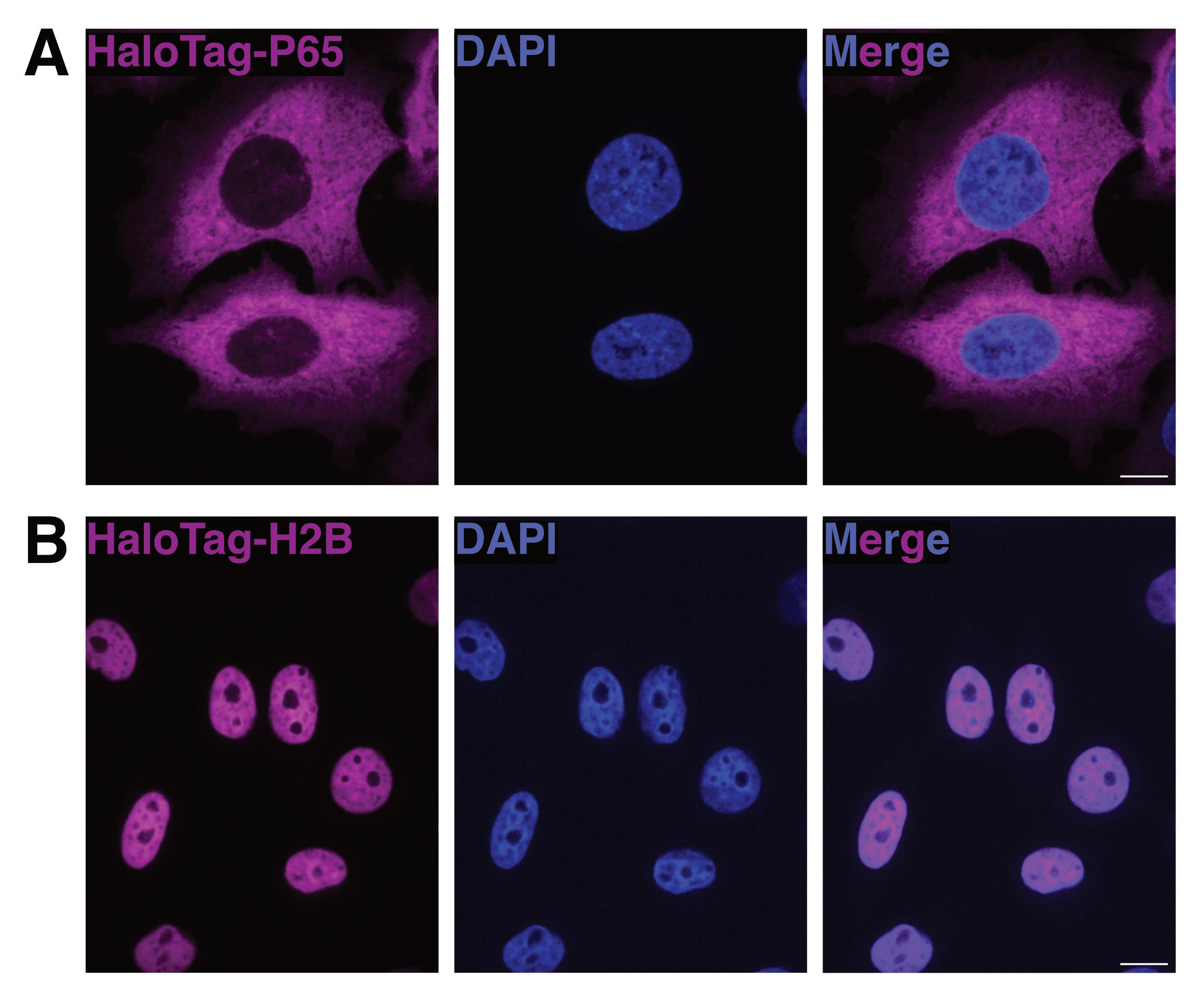
Figure 1. Visualization of HaloTag localization with fluorescence microscopy. (A) A max projected image of HeLa cells expressing cytoplasmically localized HaloTag-P65. Nuclei are counterstained with DAPI. Scale bar = 10 μm. (B) Max projected image of HeLa cells expressing nuclear-localized HaloTag-H2B. Nuclei are counterstained with DAPI. Scale bar = 10 μm.
C. Confirm the protein of interest contains a HaloTag
1. Plate ~2.2 × 10⁶ cells/dish containing the HaloTag fusion protein into two 10 cm tissue culture dishes. Cells should be around 80%–95% confluent on the day of cell lysis harvest to avoid excessive cell proliferation.
Note: The volumes listed in this protocol are for a 10 cm dish and may be adjusted up or down depending on dish size.
2. Induce expression of the HaloTag fusion protein, as described in step B3, in one of the two 10 cm dishes. Include a negative control where the HaloTag fusion protein is not induced in the other 10 cm dish.
Note: For this assay, cells with induced HaloTag fusion protein expression are compared with cells that are not induced to confirm that the expression of the HaloTag on the protein of interest is doxycycline inducible.
3. Remove the media and wash cells with 4 mL of PBS at room temperature for 1 min.
4. Remove the PBS and add 4 mL of Halo-JF buffer to each dish. Incubate in a 37 °C cell culture incubator for 15 min.
Note: Perform the remaining steps in light-reduced areas whenever possible to avoid photobleaching of the fluorophore.
5. Remove the Halo-JF buffer and wash cells twice with 4 mL of cell culture media in a 37 °C cell culture incubator for 10 min each.
6. Remove the media and wash cells twice with 4 mL of PBS in a 37 °C cell culture incubator for 10 min.
7. Remove the PBS and add 1 mL of RIPA to each dish. Scrape cells from the tissue culture dish with a cell scraper into individual 1.5 mL microcentrifuge tubes.
8. Break down the cell lysate by passing the lysate through a 20 G syringe 10–15 times.
9. Centrifuge the cell lysate at maximum speed for 5 min at 4 °C.
10. Remove the supernatant and place in a new 1.5 mL microcentrifuge tube.
11. Run the fluorescently labeled HaloTag cell lysate on a protein gel. Combine 11 μL of cell lysate with 4 μL of 4× SDS-PAGE sample buffer and 1 μL of 50 mM DTT. Heat in either a thermocycler or heat block at 95 °C for 5 min.
Note: An equal volume of cell lysis is used in this step, assuming the experimental sample and negative control sample cells are at equivalent confluency. The protein concentration of the cell lysis can be quantified through standard quantification methods [24].
12. Load a NuPAGE Bis-Tris (4%–12%) protein gel into a gel box and fill with 1× MOPS running buffer. Load 10–50 μg of protein onto the gel, including a protein ladder. Run at 120 V for 45–60 min.
13. Remove the gel from the plastic casing and place in deionized (DI) water to keep the gel hydrated.
14. Image the gel on an imager capable of detecting fluorescence in the range of the Janelia Fluor used in the experiment (Figure 2). A fluorescent band should be visible at the molecular weight of the tagged protein of interest plus the molecular weight of the HaloTag (~33 kDa).
Note: The authors used a Janelia Fluor 549 HaloTag Ligand, so the gel was imaged under the Alexa 546 setting with an intensity setting of 9. If using a different Janelia Fluor HaloTag ligand fluorophore, image at the appropriate excitation setting for that fluorophore.
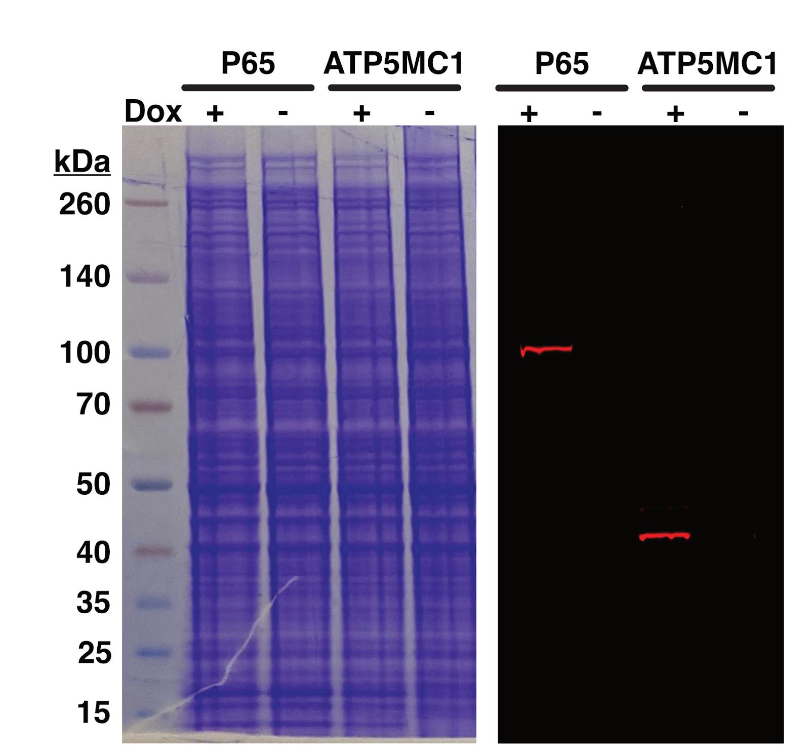
Figure 2. Confirmation of HaloTag fusion protein generation. Two HeLa cell lines expressing doxycycline-inducible HaloTag fusion proteins are visualized on a protein gel. Total protein load is visualized with Coomassie blue (left). Appendage of a HaloTag to the protein of interest is visualized with a fluorescent band (right) at the expected molecular weight of the protein plus the HaloTag (~33 kDa). Fluorescent bands are visible in a doxycycline-inducible manner for the HaloTag fusion proteins P65 (MW = 65 kDa) and ATP5MC1 (MW = 14 kDa).
15. Counterstain the gel with Coomassie Brilliant Blue for total protein detection. Place the gel in a container and add enough Coomassie Brilliant Blue stain to cover the gel. Incubate with gentle rocking for 30 min at room temperature.
Note: Coomassie Brilliant Blue staining will inform on the relative total protein content loaded into each well of the protein gel.
16. Remove the Coomassie Brilliant Blue stain from the container and add enough Coomassie destain to cover the gel. Incubate with gentle rocking overnight at room temperature.
17. Image the gel on an imager using the visible light setting.
D. Induce oxidation and isolate RNA
1. Plate ~2.2 × 10⁶ cells/dish cells containing the HaloTag fusion protein into two 10 cm tissue culture dishes. Cells should be around 80%–95% confluent on the day of cell lysis harvest to avoid excessive cell proliferation.
2. Induce expression of the HaloTag fusion protein, as described in step B3, in both the experimental sample and negative control sample for each cell line.
Note: For this procedure, both the experimental sample and negative control are induced to express the HaloTag fusion protein. Negative control samples will not contain the Halo-DBF ligand that generates free oxygen radicals to label RNAs in proximity to the HaloTagged protein of interest.
3. Remove the media and wash cells with 4 mL of PBS twice for 1 min at room temperature.
4. Remove the PBS from each dish. Add 4 mL of Halo-DBF buffer to the experimental sample and 4 mL of HBSS to the negative control sample. Incubate in a 37 °C cell culture incubator for 15 min.
Note: Perform the remaining steps in light-reduced areas whenever possible.
5. Remove the Halo-DBF buffer and wash cells twice with 4 mL of cell culture media in a 37 °C cell culture incubator for 10 min.
6. Remove the media and add 4 mL of PBS to each dish.
7. Place the cell dishes on the bottom light panel and remove the lids of the cell dishes (Figure 3). Place the second light panel on top of the cell dishes. Configure the lights to shine green light on the highest setting.
Caution: Avoid looking directly at the lights when they are turned on and use appropriate eye protection.
Caution: When placing the top light panel on the cells, be careful not to knock over the dishes.
Note: Perform this step in an area protected from light.
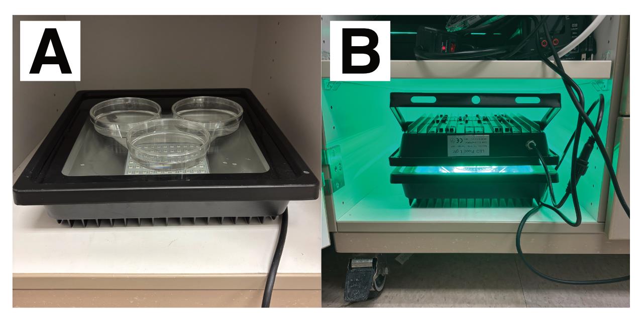
Figure 3. Light-induced labeling setup. (A) Place cell dishes on the bottom light panel and remove the lids. Three 10 cm dishes are shown. (B) Place the second light panel on top of the dishes and turn on the green lights. Protect the cells from external light by closing the cabinet door.
8. Irradiate the cells with green light on the highest setting (6,000 Lumen) for 5 min. These lights can accommodate six 6 cm dishes, three 10 cm dishes, or one 15 cm dish.
9. Remove the PBS and add 1 mL of Trizol or RNA lysis buffer (from Zymo Research kit, R1055) to the cells. Scrape cells from the tissue culture dish with a cell scraper into individual microcentrifuge tubes.
10. Break down the cell lysate by passing the lysate through a 20 G syringe 10–15 times.
Pause point: Samples can be stored in Trizol at -20 °C for up to 1 year.
11. Isolate and purify nucleic acids. If using RNA lysis buffer, proceed to step D12. If using Trizol, follow the Trizol manufacturer’s protocol for nucleic acid isolation with the following amendments:
a. Add one additional wash step with 70% ethanol for increased RNA purity.
b. Incubate samples on ice for 10 min before each wash step.
c. Resuspend RNA samples in 85 μL of nuclease-free water.
Pause point: Samples can be stored at -80 °C.
12. If using RNA lysis buffer instead of Trizol, purify RNA using the Quick-RNA Miniprep kit. Elute in 30 µL of nuclease-free water.
Note: Increase the incubation time for the on-column DNase I treatment from 15 to 30 min.
13. Quantify RNA yield with a Nanodrop.
Note: RNA yield is typically 3–10 μg for a 6 cm dish, 25–100 μg for a 10 cm dish, and 300–700 μg for a 15 cm dish.
Pause point: RNA samples can be stored at -80 °C.
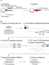
E. Library prep option 1: Targeted amplicon sequencing
1. Perform reverse transcription using a gene-specific primer for the transcript of interest. This primer should contain a unique molecular identifier (UMI) as well as a sequence that facilitates the addition of Illumina adapters. Annotated examples of reverse transcription and PCR primers are provided in Table S1. Perform the reverse transcription reaction according to the SuperScript IV reverse transcriptase protocol with 2.5 μg of RNA, with the following amendments:
a. During cDNA synthesis, incubate samples at 55 °C for 1 h instead of 10 min.
b. Near the end of the enzyme inactivation, prepare RNase buffer (see Recipes). Add 2 μL of RNase buffer to each sample and incubate at 37 °C for 30 min.
Note: A control reaction without reverse transcriptase serves as a negative control to assess for DNA contamination in the purified RNA samples.
2. Prepare cDNA samples for PCR using gene-specific forward and reverse primers that contain Illumina-capable sequencing adapters. Annotated examples of reverse transcription and PCR primers are provided in Table S1. Use 3 μL of cDNA per 25 μL of PCR reaction, which results in seven PCR reactions per sample.
Note: Gene-specific forward and reverse primers used at this step include Illumina-capable sequencing adapters appended to the primers. This allows for Illumina sequencing directly after eluting the library from the final bead clean-up step.
3. Perform PCR according to the protocol described in Table 1.
Critical: Determine the appropriate annealing temperature and number of cycles necessary to generate an amplicon by performing PCR titrations for each set of primers for the gene. Choose the annealing temperature and the lowest cycle number that reliably generates a product visible by agarose gel electrophoresis. Use these values for the amplicon-specific temperature and cycle number listed in Table 1. If 10 cycles at the amplicon-specific annealing temperature are not enough to generate a detectable amplicon, then additional cycles using an annealing temperature of 72 °C should be included to generate an amplicon product.
Table 1. PCR program for the generation of targeted amplicon libraries
| Step | Temperature | Time | Cycles |
| Denaturation | 98 °C | 30 s | |
| Denaturation | 98 °C | 30 s | 10× |
| Anneal | Amplicon-specific | 30 s | |
| Extension | 72 °C | 15 s | |
| Denaturation | 98 °C | 30 s | Amplicon-specific (0–15×) |
| Anneal | 72 °C | 30 s | |
| Extension | 72 °C | 15 s | |
| Final extension | 72 °C | 60 s | |
| Hold | 4 °C |
4. Pool together all PCR reactions for each sample into a new 1.5 mL microcentrifuge tube.
5. Clean up the samples using DNA Clean and Concentrator-5. Elute in 40 μL of DNA elution buffer twice for a total of ~80 μL of eluted DNA per sample.
6. Bring PCR clean-up reactions to 100 μL per sample with DNA elution buffer.
7. Add 80 μL of KAPA Pure Beads (0.8× clean-up) to each sample and mix by vortexing gently. Incubate at room temperature for 15 min with occasional flicking.
Note: The ratio of KAPA Pure Beads to RNA sample during this step can impact the size selection of the final library. Refer to the KAPA Pure Beads technical data sheet for more information.
8. Place on a magnet and incubate at room temperature for 1 min on the magnetic tube rack. Remove the supernatant from the beads and discard.
9. Add 200 μL of 80% ethanol to each tube and incubate at room temperature for 30 s on the magnetic tube rack.
10. Keeping the tubes on the magnetic rack, carefully remove the ethanol from each tube. Add 200 μL of 80% ethanol to each tube and incubate at room temperature for 30 s on the magnetic tube rack.
11. Remove the ethanol from each tube and keep the tubes on the magnetic tube rack. Allow the beads to dry for ~3–5 min.
12. Remove the tubes from the magnetic rack and resuspend each tube in 20 μL of 10 mM Tris pH 8.0. Incubate at room temperature for 2 min.
13. Place tubes on a magnetic rack and incubate at room temperature for 1 min.
14. Carefully remove the supernatant from the beads and place in a new microcentrifuge tube. This is the eluted library.
F. Library prep option 2: Total mRNA sequencing
1. Prepare RNA libraries according to the Lexogen QuantSeq 3’ mRNA-Seq Library Prep kit instructions.
Notes:
1. This library prep kit selects for polyadenylated mRNAs. If the mRNAs of interest are not polyadenylated, using a targeted approach or Halo-seq may be more appropriate for proximity labeling.
2. Detecting mutations with both reads of a mate pair increases confidence in mutation calling. This requires that during library preparation, insert sizes are approximately the length of the read that will be used in the resulting RNAseq reaction. For example, we often use paired-end 150 bp reactions. We therefore aim for insert sizes of approximately 200–250 nt.
G. Perform quality control on the libraries prior to sequencing
1. Determine the concentration of each library using the Qubit RNA HS Assay kit according to the Qubit instructions, using 1 μL per sample.
Note: Library concentrations above 1 ng/μL are sufficient for sequencing.
2. Determine the size distribution of the library fragments by running each library on a Tapestation using 1 μL per sample.
Note: For detection of nucleotide conversions in both reads of paired-end sequencing, the mean library size should not exceed ~250 bp.
3. Submit for high-throughput sequencing.
Data analysis
During the OINC-seq procedure, guanosine residues in RNA that are proximal to the HaloTag protein are oxidized. These oxidized residues are misinterpreted by reverse transcriptase, leading to G to T, G to C, and G deletion mutations in the resulting cDNA. The frequency of these mutations in a given RNA species is therefore a readout of its proximity to the HaloTag bait.
In order to quantify these mutations for each gene, we have created the Pipeline for the Identification of Guanosine Positions Erroneously Notated, or PIGPEN, software package. This section will describe the installation and usage of PIGPEN as well as the interpretation of its output.
Installation
PIGPEN is only available for Linux operating systems. It is installable either by using the Python package manager conda or directly from GitHub. There are no specific requirements in terms of memory and analysis power to run this package, although access to a cluster with multiple processors will allow it to run faster.
A. Installation via the conda package manager
1. If not done already, install the conda package manager (https://docs.conda.io/projects/conda/en/latest/user-guide/install/index.html).
2. Add the Bioconda channel to your conda installation by running the following commands:
conda config –add channels biocondaconda config –add channels conda-forgeconda config –set channel_priority strict3. Create a new environment using conda create -n pigpen_env
4. Enter the new pigpen environment using source activate pigpen_env
5. Install PIGPEN using conda install -c bioconda pigpen
B. Installation from GitHub repository
1. If not done already, install the conda package manager (https://docs.conda.io/projects/conda/en/latest/user-guide/install/index.html).
2. Download pigpen_env.yaml from https://github.com/TaliaferroLab/OINC-seq.
3. Create a conda environment called pigpen_env using conda env create -f pigpen_env.yaml
4. Enter the new pigpen environment using source activate pigpen_env
5. Download PIGPEN using wget https://github.com/TaliaferroLab/OINC-seq/archive/refs/heads/master.zip
6. Decompress this directory using unzip master.zip
7. Enter the PIGPEN directory using cd OINC-seq-master
8. Install PIGPEN using python setup.py install
Analyzing OINC-seq data with PIGPEN
As outlined in the experimental procedures above, PIGPEN can either interrogate whole transcriptomes through RNAseq libraries or single transcripts through amplicon sequencing. For both approaches, reads are first aligned to the transcriptome using STAR [25] and RNA abundances are quantified using salmon [26].
Single-nucleotide polymorphisms (SNPs) are indistinguishable from oxidation-induced mutations but do not report on RNA localization. They therefore need to be excluded from RNA localization quantifications. PIGPEN performs this by calling SNPs relative to a reference genome [27] in control samples that did not receive oxidation-inducing treatments (e.g., samples in which Halo-DBF or green light treatment was omitted). By default, genomic locations containing SNPs supported by at least 20 reads and at a frequency of at least 40% are excluded from downstream analyses. Optionally, user-defined locations can be masked as well.
After running PIGPEN, a table is produced that contains mutation rates for all genes (in the case of whole transcriptome samples) or each user-defined region (in the case of amplicon-based experiments).
A. Trim sequencing adapters from reads
1. For whole transcriptome experiments, adapters are trimmed with Cutadapt [28]. A multistep strategy for trimming adapters from Lexogen Quantseq libraries can be found at https://github.com/TaliaferroLab/OINC-seq/blob/master/cutadapt.sh.
2. For amplicon experiments, if read sequences contain adapter sequences, then adapters should be trimmed. However, the size and sequence content of these adapters will depend on their design.
B. Align reads to the transcriptome and quantify RNA abundances
These steps are done automatically through the use of the alignAndQuant tool included with PIGPEN.
1. The alignAndQuant tool can be run using the following command: alignAndQuant <options>
a. --forwardreads Gzipped fastq file containing forward reads (i.e., R1 of a paired-end sequencing run).
b. --reversereads Gzipped fastq file containing reverse reads (i.e., R2 of a paired-end sequencing run). Do not supply this option if using single-end reads.
c. --nthreads Number of threads to use for alignment and quantification.
d. --STARindex Directory containing STAR alignment index for the genome of interest. This can be produced using STAR, which is automatically installed during PIGPEN installation. For more information, see https://github.com/alexdobin/STAR/blob/master/doc/STARmanual.pdf.
e. --salmonindex Directory containing salmon index for quantification of the transcriptome of interest. This can be produced using salmon, which is automatically installed during PIGPEN installation. For more information, see https://salmon.readthedocs.io/en/latest/.
f. --samplename Name of the sample.
g. --maxmap Maximum number of allowable alignments for a read. Reads that align to more places than this in the genome will be ignored. This reduces spurious mutations that arise due to poor alignment.
2. After running alignAndQuant, the data for each sample will be contained within a directory named samplename. Each directory will contain the transcriptomic alignment produced by STAR and the transcriptome quantification produced by salmon. The architecture of this directory is important as its specific organization is expected by PIGPEN.
C. Quantify mutations in RNAseq data using PIGPEN
This step will automatically identify and mask SNPs (if desired). For transcriptome-wide experiments, it will output a table of mutation rates for each gene. For amplicon experiments, it will output a table for each region of interest.
1. PIGPEN can be run using the following command: pigpen <options>
a. --datatype Either “single” or “paired,” depending on whether the supplied data is single-end or paired-end.
b. --samplenames Comma-separated list (without spaces) of samples to quantify. These should correspond to the sample names used in the call to alignAndQuant and should therefore also correspond to directory names in the current working directory.
c. --controlsamples Comma-separated list (without spaces) of control samples (i.e., those where no induced conversions are expected). This may be a sublist of the list provided to --samplenames.
d. -gff Genome annotation in gff format. Annotations from GENCODE or Ensembl are strongly preferred.
e. --genomeFasta Genome sequence in fasta format. Required if SNPs are to be considered.
f. --nproc Number of processors to use. Default is 1.
g. --useSNPs Supply this option if you want to identify and mask SNPs using --controlsamples.
h. --maskbed This is an optional bed file of additional sites to mask from mutation quantification.
i. --ROIbed This is an optional bed file of specific regions of interest in which to quantify conversions. If supplied, only conversions in these regions will be quantified. It is most useful when defining an amplicon in which mutations should be quantified.
j. --SNPcoverage The minimum read coverage with which to call a SNP. The default is 20.
k. --SNPfreq The minimum variant frequency with which to call a SNP. The default is 0.4.
l. --onlyConsiderOverlap Supply this option if you only want to consider mutations seen in both reads of a read pair. This option is only relevant when using paired-end data and greatly reduces background mutation rates.
m. --use_g_t Supply this option if you want to consider G to T mutations when calculating overall mutation rates.
n. --use_g_c Supply this option if you want to consider G to C mutations when calculating overall mutation rates.
o. --use_g_x Supply this option if you want to consider G deletion mutations when calculating overall mutation rates.
p. --use_read1 Supply this option if you want to use read 1 when looking for mutations. This is only relevant with paired-end data, and the usage of –-onlyConsiderOverlap requires the usage of both read 1 and read 2.
q. --use_read2 Supply this option if you want to use read 2 when looking for mutations. This is only relevant with paired-end data, and the usage of –-onlyConsiderOverlap requires the usage of both read 1 and read 2.
r. --minMappingQual The minimum transcriptome alignment quality for a read to be considered in mutation counting.
s. --minPhred The minimum phred quality score for a base to be considered when counting mutations.
t. --nConv The minimum number of mutations (defined by –use_g_t, –use_g_c, and –use_g_x options above) in a read or read pair in order for those mutations to be counted.
u. --outputDir Output directory.
2. PIGPEN may take several hours to complete, depending on the number of reads in the experiment. The usage of multiple processors greatly reduces running time.
3. After completion, one table of mutation rates for every gene or amplicon will be produced for each sample and placed in --outputDir.
D. Identify genes with differences in mutation rates across conditions using the bioinformatic analysis of the conversion of nucleotides (BACON) module
1. To identify genes whose mutation rates significantly vary across samples or conditions, BACON fits a binomial generalized linear mixed effects model of counts of mutated and nonmutated G residues across conditions. This model is then compared to a null model in which the effect of the condition is removed. To evaluate the relative fit between the experimental and null models, a likelihood ratio test is then used. P values derived from this likelihood ratio test are then corrected for multiple hypothesis testing and reported as FDR (false discovery rate) values.
2. BACON requires a standardized file that relates PIGPEN output files, the samples they belong to, and the conditions they belong to. These are three columns, tab-delimited files with the column names “file,” “sample,” and “condition.” For each sample, the file column refers to the PIGPEN output file associated with that sample, the sample column refers to the name of the sample, and the condition column refers to the condition the sample belongs to.
3. BACON can be run using the following command: bacon <options>
a. --sampconds Path to the file described in section B above that relates sample IDs, the conditions that samples belong to, and their associated PIGPEN output files.
b. --minreads The minimum read count for a gene in order for its mutation rate to be quantified. The default is 100.
c. --conditionA One of the two conditions in the “condition” column of the sampconds file. Differences in mutation rates between samples will be reported as conditionB - condition A.
d. --conditionB One of the two conditions in the “condition” column of the sampconds file. Differences in mutation rates between samples will be reported as conditionB - condition A.
e. --use_g_t Supply this option if you want to consider G to T mutations when comparing mutation rates across samples.
f. --use_g_c Supply this option if you want to consider G to C mutations when comparing mutation rates across samples.
g. --use_g_x Supply this option if you want to consider G deletion mutations when comparing mutation rates across samples.
h. --output Output file.
4. Generally, BACON will take 5–30 min to complete running. After completing, it will generate a table of mutation rates in each sample, differences in those mutation rates across conditions, and P and FDR values for those differences for all genes.
Validation of protocol
OINC-seq and PIGPEN were benchmarked by assaying their ability to report on the spatial distribution of RNAs with known localization patterns. In the publication first describing OINC-seq [17], the localization of GAPDH and MALAT1 transcripts, which are known to be primarily cytoplasmic and nuclear, respectively, was assayed using OINC-seq. These known patterns were recapitulated with OINC-seq (see Figure 3 of [17]). Similarly, for transcriptome-wide experiments, RNA classes known to be enriched at different locations were again used as positive controls. For example, mRNAs encoding secreted peptides are preferentially translated on the surface of the endoplasmic reticulum in order to facilitate protein sorting and secretion. Using an ER-localized bait protein, these mRNAs were again found to be predominantly ER-proximal by OINC-seq, further validating the method (see Figure 4 of [17]).
For validation of data analysis using PIGPEN, OINC-seq datasets and associated PIGPEN output files for several samples are available at the Gene Expression Omnibus: https://www.ncbi.nlm.nih.gov/geo/query/acc.cgi?acc=GSE279714
This protocol has been used and validated in the following research article(s):
• Lo et al. [17] Quantification of subcellular RNA localization through direct detection of RNA oxidation. Nucleic Acids Res., 53(5), gkaf139. https://doi.org/10.1093/nar/gkaf139
General notes and troubleshooting
General notes
1. Not all reverse transcriptase enzymes generate detectable mutations in oxidized guanosine residues. SuperScript IV reverse transcriptase and the proprietary reverse transcriptase included in the Lexogen QuantSeq 3′ mRNA-Seq Library Prep kit FWD generate mutations at oxidized guanosine residues with low levels of background mutations. Other polymerases may be suitable for OINC-seq but have not been tested.
2. Total mRNA sequencing using the Lexogen QuantSeq 3′ mRNA-Seq Library kit FWD utilizes oligo(dT) primers to generate cDNA. If some transcripts of interest are not polyadenylated, a targeted approach with gene-specific primers or Halo-seq may be a more appropriate method to assess localization.
Troubleshooting
Problem 1: Cell viability is decreased upon the addition of a HaloTag.
Possible cause: The addition of a HaloTag affects the functionality of the protein of interest.
Solution: Append the HaloTag to the alternate terminus of the protein of interest and reassess cell viability. If the addition of a HaloTag to the endogenous protein affects cell viability, switch to an inducible expression system.
Problem 2: HaloTag is not localized to the expected subcellular location.
Possible cause: The addition of a HaloTag domain to the protein of interest may alter the protein’s ability to localize.
Solution: Append the HaloTag to the alternate terminus of the protein and reassess its subcellular localization.
Problem 3: HaloTag is not visible during fluorescent microscopy imaging.
Possible cause: The protein of interest containing the HaloTag is lowly expressed.
Solution: Run cell lysis on a Halo gel to confirm that the protein of interest is successfully HaloTagged. Generate a positive control cell line by appending a HaloTag to a highly expressed protein.
Supplementary information
The following supporting information can be downloaded here:
1. Table S1. Example primers for Illumina-based sequencing of OINC-seq amplicons.
Acknowledgments
We wish to acknowledge Agnese Kocere, Joelle Lo, Laura White, Haydee Ramirez, Abraham Martinez, Seth Jacobson, Chad Pearson, Marino Resendiz, and Christian Mosimann for their help in the development of OINC-seq. We further acknowledge Ying Li and Robert Spitale for their help in the development of the predecessor method Halo-seq, as well as for the synthesis of Halo-DBF. We acknowledge Rob Patro for his help in developing Postmaster software for the fractional assignment of RNA-seq reads to transcripts. This work was supported by NIH grant R35-GM133385 and by funding from the W.M. Keck Foundation. This protocol was used in [17].
Competing interests
The authors declare no conflicts of interest.
References
- Long, R. M., Singer, R. H., Meng, X., Gonzalez, I., Nasmyth, K. and Jansen, R. P. (1997). Mating type switching in yeast controlled by asymmetric localization of ASH1 mRNA. Science. 277(5324): 383–387. https://doi.org/10.1126/science.277.5324.383
- Ephrussi, A., Dickinson, L. K. and Lehmann, R. (1991). Oskar organizes the germ plasm and directs localization of the posterior determinant nanos. Cell. 66(1): 37–50. https://doi.org/10.1016/0092-8674(91)90137-n
- Ephrussi, A. and Lehmann, R. (1992). Induction of germ cell formation by oskar. Nature. 358(6385): 387–392. https://doi.org/10.1038/358387a0
- Goering, R., Hudish, L. I., Guzman, B. B., Raj, N., Bassell, G. J., Russ, H. A., Dominguez, D. and Taliaferro, J. M. (2020). FMRP promotes RNA localization to neuronal projections through interactions between its RGG domain and G-quadruplex RNA sequences. eLife. 9: e52621. https://doi.org/10.7554/elife.52621
- Wang, E. T., Taliaferro, J. M., Lee, J.-A., Sudhakaran, I. P., Rossoll, W., Gross, C., Moss, K. R. and Bassell, G. J. (2016). Dysregulation of mRNA localization and translation in genetic disease. J Neurosci. 36(45): 11418–11426. https://doi.org/10.1523/JNEUROSCI.2352-16.2016
- Adekunle, D. A. and Wang, E. T. (2020). Transcriptome-wide organization of subcellular microenvironments revealed by ATLAS-Seq. Nucleic Acids Res. 48(11): 5859–5872. https://doi.org/10.1093/nar/gkaa334
- Arora, A., Goering, R., Lo, H.-Y. G. and Taliaferro, M. J. (2021). Mechanical fractionation of cultured neuronal cells into cell body and neurite fractions. Bio Protoc. 11(11): e4048. https://doi.org/10.21769/BioProtoc.4048
- Blower, M. D., Feric, E., Weis, K. and Heald, R. (2007). Genome-wide analysis demonstrates conserved localization of messenger RNAs to mitotic microtubules. J Cell Biol. 179(7): 1365–1373. https://doi.org/10.1083/jcb.200705163
- Ciolli Mattioli, C., Rom, A., Franke, V., Imami, K., Arrey, G., Terne, M., Woehler, A., Akalin, A., Ulitsky, I. and Chekulaeva, M. (2019). Alternative 3’ UTRs direct localization of functionally diverse protein isoforms in neuronal compartments. Nucleic Acids Res. 47(5): 2560–2573. https://doi.org/10.1093/nar/gky1270
- Farmer, T., Vaeth, K. F., Han, K.-J., Goering, R., Taliaferro, M. J. and Prekeris, R. (2023). The role of midbody-associated mRNAs in regulating abscission. J Cell Biol. 222(12): e202306123. https://doi.org/10.1083/jcb.202306123
- Taliaferro, J. M., Vidaki, M., Oliveira, R., Olson, S., Zhan, L., Saxena, T., Wang, E. T., Graveley, B. R., Gertler, F. B., Swanson, M. S., et al. (2016). Distal alternative last exons localize mRNAs to neural projections. Mol Cell. 61(6): 821–833. https://doi.org/10.1016/j.molcel.2016.01.020
- Wang, E. T., Cody, N. A. L., Jog, S., Biancolella, M., Wang, T. T., Treacy, D. J., Luo, S., Schroth, G. P., Housman, D. E., Reddy, S., et al. (2012). Transcriptome-wide regulation of pre-mRNA splicing and mRNA localization by muscleblind proteins. Cell. 150(4): 710–724. https://doi.org/10.1016/j.cell.2012.06.041
- Engel, K. L., Lo, H.-Y. G., Goering, R., Li, Y., Spitale, R. C. and Taliaferro, J. M. (2022). Analysis of subcellular transcriptomes by RNA proximity labeling with Halo-seq. Nucleic Acids Res. 50(4): e24. https://doi.org/10.1093/nar/gkab1185
- Fazal, F. M., Han, S., Parker, K. R., Kaewsapsak, P., Xu, J., Boettiger, A. N., Chang, H. Y. and Ting, A. Y. (2019). Atlas of subcellular RNA localization revealed by APEX-seq. Cell. 178(2): 473-490.e26. https://doi.org/10.1016/j.cell.2019.05.027
- Padrón, A., Iwasaki, S. and Ingolia, N. T. (2019). Proximity RNA labeling by APEX-seq reveals the organization of translation initiation complexes and repressive RNA granules. Mol Cell. 75(4): 875–887.e5. https://doi.org/10.1016/j.molcel.2019.07.030
- Wang, P., Tang, W., Li, Z., Zou, Z., Zhou, Y., Li, R., Xiong, T., Wang, J. and Zou, P. (2019). Mapping spatial transcriptome with light-activated proximity-dependent RNA labeling. Nat Chem Biol. 15(11): 1110–1119. https://doi.org/10.1038/s41589-019-0368-5
- Lo, H.-Y. G., Goering, R., Kocere, A., Lo, J., Pockalny, M. C., White, L. K., Ramirez, H., Martinez, A., Jacobson, S., Spitale, R. C., et al. (2025). Quantification of subcellular RNA localization through direct detection of RNA oxidation. Nucleic Acids Res. 53(5): gkaf139. https://doi.org/10.1093/nar/gkaf139
- Los, G. V., Encell, L. P., McDougall, M. G., Hartzell, D. D., Karassina, N., Zimprich, C., Wood, M. G., Learish, R., Ohana, R. F., Urh, M., et al. (2008). HaloTag: a novel protein labeling technology for cell imaging and protein analysis. ACS Chem Biol. 3(6): 373–382. https://doi.org/10.1021/cb800025k
- Alenko, A., Fleming, A. M. and Burrows, C. J. (2017). Reverse transcription past products of guanine oxidation in RNA leads to insertion of A and C opposite 8-oxo-7,8-dihydroguanine and A and G opposite 5-guanidinohydantoin and spiroiminodihydantoin diastereomers. Biochemistry. 56(38): 5053–5064. https://doi.org/10.1021/acs.biochem.7b00730
- Li, Y., Aggarwal, M. B., Ke, K., Nguyen, K. and Spitale, R. C. (2018). Improved analysis of RNA localization by spatially restricted oxidation of RNA-protein complexes. Biochemistry. 57(10): 1577–1581. https://doi.org/10.1021/acs.biochem.8b00053
- Khandelia, P., Yap, K. and Makeyev, E. V. (2011). Streamlined platform for short hairpin RNA interference and transgenesis in cultured mammalian cells. Proc Natl Acad Sci USA. 108(31): 12799–12804. https://doi.org/10.1073/pnas.1103532108
- McCornack M., Schagat T. and Slater M. (2008). Expression of Fusion Proteins: How to Get Started with the HaloTag® Technology. Promega Notes. 100. Retrieved from https://www.promega.com/-/media/files/resources/promega-notes/100/expression-of-fusion-proteins-how-to-get-started-with-the-halotag-technology.pdf?rev=8694aa6307214e80a014fefb8d7b0104&sc_lang=en
- Goyal, G. (2019). Basic immunofluorescence protocol for adherent cells v1. Data set. In protocols.io. ZappyLab, Inc. https://doi.org/10.17504/protocols.io.wt4feqw
- Noble, J. E. and Bailey, M. J. A. (2009). Quantitation of protein. Methods Enzymol. 463: 73–95. https://doi.org/10.1016/S0076-6879(09)63008-1
- Dobin, A., Davis, C. A., Schlesinger, F., Drenkow, J., Zaleski, C., Jha, S., Batut, P., Chaisson, M. and Gingeras, T. R. (2013). STAR: ultrafast universal RNA-seq aligner. Bioinformatics. 29(1): 15–21. https://doi.org/10.1093/bioinformatics/bts635
- Patro, R., Duggal, G., Love, M. I., Irizarry, R. A. and Kingsford, C. (2017). Salmon provides fast and bias-aware quantification of transcript expression. Nat Methods. 14(4): 417–419. https://doi.org/10.1038/nmeth.4197
- Koboldt, D. C., Chen, K., Wylie, T., Larson, D. E., McLellan, M. D., Mardis, E. R., Weinstock, G. M., Wilson, R. K. and Ding, L. (2009). VarScan: variant detection in massively parallel sequencing of individual and pooled samples. Bioinformatics. 25(17): 2283–2285. https://doi.org/10.1093/bioinformatics/btp373
- Martin, M. (2011). Cutadapt removes adapter sequences from high-throughput sequencing reads. EMBnet.journal. 17(1): 10–12. https://doi.org/10.14806/EJ.17.1.200
Article Information
Publication history
Received: May 9, 2025
Accepted: Jun 24, 2025
Available online: Jul 22, 2025
Published: Aug 5, 2025
Copyright
© 2025 The Author(s); This is an open access article under the CC BY-NC license (https://creativecommons.org/licenses/by-nc/4.0/).
How to cite
Pockalny, M. C., Lo, H.-Y. G., Goering, R. and Taliaferro, J. M. (2025). Analyzing RNA Localization Using the RNA Proximity Labeling Method OINC-seq. Bio-protocol 15(15): e5403. DOI: 10.21769/BioProtoc.5403.
Category
Bioinformatics and Computational Biology
Molecular Biology > RNA > RNA localisation
Molecular Biology > RNA > RNA sequencing
Do you have any questions about this protocol?
Post your question to gather feedback from the community. We will also invite the authors of this article to respond.