- Protocols

- Articles and Issues
- For Authors
- About
- Become a Reviewer

Evaluating Arabidopsis Primary Root Growth in Response to Osmotic Stress Using an In Vitro Osmotic Gradient Experimental System
Published: Vol 15, Iss 14, Jul 20, 2025 DOI: 10.21769/BioProtoc.5397 Views: 1939
Reviewed by: Tohir A. BozorovAnonymous reviewer(s)
Original research article
The authors used this protocol in:

Nov 2024

Protocol Collections
Comprehensive collections of detailed, peer-reviewed protocols focusing on specific topics


Related protocols
Abstract
The root meristem navigates the highly variable soil environment where water availability limits water absorption, slowing or halting growth. Traditional studies use uniform high osmotic potentials, poorly representing natural conditions where roots gradually encounter increasing osmotic potentials. Uniform high osmotic potentials reduce root growth by inhibiting cell division and shortening mature cell length. This protocol describes a simple and effective in vitro system using a gradient mixer that generates a vertical gradient in an agar gel based on the principle of communicating vessels, exploiting gravity to generate a continuous mannitol concentration gradient (from 0 to 400 mM mannitol) reaching osmotic potentials of -1,2 MPa. It enables long-term Arabidopsis root growth analysis under progressive water deficit, improving phenotyping and molecular studies in soil-like conditions.
Key features
• Novel approach: Unique method to evaluate primary root growth in Arabidopsis under increasing osmotic potentials.
• Osmotic gradient system: Simulating a gradual osmotic gradient in the root growth zone while maintaining aerial tissues under control conditions.
• Sustained growth: Arabidopsis Col-0 and ttl1 mutant seedlings maintain proper root growth for 25 days, even at osmotic potentials as low as -1.2 MPa.
• Enhanced growth rates: Roots grown in the osmotic gradient exhibit higher growth rates than those in homogeneous high osmotic potential conditions.
• Phenotypic observation: ttl1 seedlings grown in the osmotic gradient do not show the typical swelling phenotype observed at extreme osmotic potentials (-1.2 MPa).
Keywords: Osmotic gradientGraphical overview
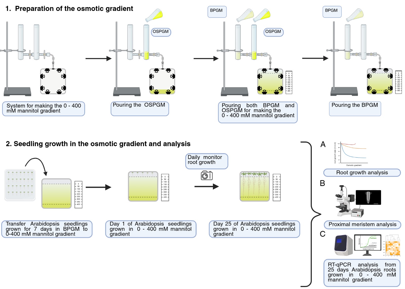
Graphical overview of the root growth analysis during osmotic stress in an in vitro osmotic gradient experimental system. BPGM: basic plant growth media; OSPMG: osmotic shock plant growth media.
Background
The root meristem faces probably one of the most complex environments on Earth: the soil, whose physicochemical properties can vary dramatically on a micrometer scale, exposing roots to various types of stress, such as osmotic stress [1]. Osmotic stress limits the ability of cells to absorb water, causing growth delay or arrest. Most studies aimed at understanding root growth adaptation to osmotic stress use homogeneous high osmotic potentials (osmotic shock) on shoots and roots [2–4]. However, this approach does not accurately mimic natural field conditions, where roots encounter progressively increasing osmotic potentials while navigating the soil. Osmotic shock significantly inhibits root growth by reducing cell division in the proximal meristem and shortening mature cell length [5]. Here, we present an efficient and straightforward protocol to generate an in vitro osmotic gradient experimental system with increasing osmotic potentials. This protocol describes a simple and effective in vitro system using a gradient mixer that generates a vertical gradient in an agar gel based on the principle of communicating vessels, exploiting gravity to generate a continuous mannitol concentration gradient (from 0 to 400 mM mannitol), reaching osmotic potentials of -1,2 MPa. The system generates a controlled osmotic gradient in the root zone while exposing the aerial tissue to control conditions. Although the use of mannitol can be discussed due to its potential toxicity, the use of high-molecular-weight polyethylene glycol, which may more closely resemble the physiological effect of drought [6], is impossible because of its incompatibility with melted agar. The gradient system has proven valuable in quantifying germination and sustained primary root growth of Arabidopsis for 25 days under continuous conditions of decreasing water availability [7]. The system could present difficulties if working for long periods because of its semi-sterile nature. The protocol paves the way for fine-tuning phenotyping and conducting molecular studies under conditions that better simulate growth in a continuum of increasing water deficit. Moreover, in the future, there will be new opportunities for studying other forms of abiotic stresses, with the modification of the described technique to create different forms of gradients.
Materials and reagents
Biological materials
1. Columbia-0 (Col-0) was used as the wild-type genotype (TAIR)
2. TTL1 (AT1G53300), T-DNA insertion line Salk (Institute Genomic Analysis Laboratory, SALK_063943 /USA)
Reagents
1. D-Mannitol (AMRESCO, catalog number: 0122)
2. Murashige and Skoog basal salt mixture (Duchefa Biocheime, catalog number: M0221.0050)
3. TRIzolTM (Invitrogen, catalog number: 15596026); store at 4 °C
4. Plant agar (Duchefa Biocheime, catalog number: P1001.1000)
5. Sucrose (Azúcar Bella Unión, catalog number: 7730106005113)
6. Kit SuperScript® IV reverse transcriptase (Invitrogen, catalog number: 18090050) using oligo d(T)20; store at -20 °C
7. DNase I (RNase-free) (NEB, catalog number: M0303S); store at -20 °C
8. PowerUpTM SYBRTM Green Master Mix (2×) (Applied Biosystems, catalog number: A25742, USA); store at 4 °C
9. EDTA disodium (Sigma-Aldrich, catalog number: 03677)
10. Ultrapure Tris (Invitrogen, catalog number: 15504-020)
11. Glacial acetic acid (Dorwill, catalog number: DA01-05-03)
12. Water for molecular biology, nuclease-free (NZYtech, catalog number: MB11101); store at 4 °C
13. RNase AWAYTM reagent (Invitrogen, catalog number: 10328011); store at room temperature
14. SyberTM Safe DNA gel stain (Invitrogen, catalog number: S33102); store at room temperature
15. TopVision agarose (Thermo, catalog number: R0492)
16. Absolute pure ethanol (Dorwil, catalog number 4403); store at -20 °C
17. TWEEN® 20 (Sigma, catalog number: P1379-100mL)
18. Sodium hypochlorite 36% (Droguería Industrial, catalog number: 10429)
19. Chloral hydrate (Sigma-Aldrich, catalog number: C8383); store in a cool, dry, well-ventilated area in a tightly closed container in an amber bottle
20. Glycerin (Sigma-Aldrich, catalog number: G5516); store in a well-sealed container at room temperature
21. Gum Arabic (Sigma-Aldrich, catalog number: G9752); store in a dry container at room temperature
22. Sterile gauze
23. Congo Red dye (Sigma-Aldrich, catalog number: C6767)
Solutions
1. Basic plant growth media (BPGM) (see Recipes)
2. Osmotic shock plant growth media (OSPGM) (see Recipes)
3. EDTA 0.5 M (see Recipes)
4. TAE 50× (see Recipes)
5. TAE 1× (see Recipes)
6. RT-qPCR reaction composition (see Recipes)
7. Agarose gel 1% (see Recipes)
8. Ethanol 70% (see Recipes)
9. Hoyer’s solution (see Recipes)
10. Sodium hypochlorite 20% (See Recipes)
Recipes
1. Basic plant growth media (BPGM) (300 mL) pH 5.7
| Reagent | Final concentration | Quantity or Volume |
|---|---|---|
| Murashige-Skoog basal salts (4.3 g/L) | 1× | 1.29 g |
| Plant agar | 1.2% | 3.6 g |
| Sucrose | 1.5% | 4.5 g |
| Distilled water | n/a | Up to 300 mL |
2. Osmotic shock plant growth media (OSPGM) (300 mL) pH 5.7
| Reagent | Final concentration | Quantity or Volume |
|---|---|---|
| Murashige-Skoog basal salts (4.3 g/L) | 1× | 1.29 g |
| Plant agar | 1.2% | 3.6 g |
| Sucrose | 1.5% | 4.5 g |
| Mannitol | 400 mM | 21.86 g |
| Distilled water | n/a | Up to 300 mL |
3. EDTA 0.5 M (250 mL)
| Reagent | Final concentration | Quantity or Volume |
|---|---|---|
| EDTA | 0.5 M | 46.53 g |
| Distilled water | n/a | Up to 250 mL |
Adjust to pH 8 with NaOH.
4. TAE 50× (1 L)
| Reagent | Final concentration | Quantity or Volume |
|---|---|---|
| Ultrapure Tris | 2 M | 242 g |
| Glacial acetic acid | 1 M | 57.1 mL |
| EDTA 0.5 M (pH 8) | 0.05 M | 100 mL |
| Distilled water | n/a | Up to 1,000 mL |
5. TAE 1× (1 L)
| Reagent | Final concentration | Quantity or Volume |
|---|---|---|
| TAE 50× | 1× | 20 mL |
| Distilled water | n/a | 980 mL |
6. RT-qPCR reaction composition (1 reaction of 10 μL)
| Reagent | Final concentration | Quantity or Volume |
|---|---|---|
| PowerUpTM SYBRTM Green Master Mix (2×) | 1× | 5 μL |
| 10 μM forward primer | 0.6 μM | 0.6 μL |
| 10 μM reverse primer | 0.6 μM | 0.6 μL |
| cDNA | ≤500 ng | 1 μL |
| Nuclease-free water | n/a | 2.8 μL |
| Total | n/a | 10 μL |
7. Agarose gel 1% (100 mL)
| Reagent | Final concentration | Quantity or Volume |
|---|---|---|
| Top Vision Agarose | 1% | 1 g |
| 1× TAE | n/a | 100 mL |
| SYBRTM Safe (10,000×) | 0.4× | 4 μL |
8. Ethanol 70% (1L)
| Reagent | Final concentration | Quantity or Volume |
|---|---|---|
| Absolute pure ethanol | 70% | 700 mL |
| Distilled water | n/a | 300 mL |
9. Hoyer’s solution (100 mL)
| Reagent | Final concentration | Quantity or Volume |
|---|---|---|
| Chloral hydrate | 200% | 200 g |
| Gum Arabic | 30% w/v | 30 g |
| Glycerin | 20% | 20 mL |
| Distilled water | n/a | Up to 100 mL |
Store the prepared mix in a tightly sealed amber glass bottle to prevent light exposure at room temperature (around 20–25 °C) for several months.
10. 20% sodium hypochlorite
| Reagent | Final concentration | Quantity or Volume |
|---|---|---|
| Sodium hypochlorite (36%) | 7.2% | 10 mL |
| Distilled water | n/a | Up to 50 mL |
| TWEEN 20 | n/a | 10 μL |
Laboratory supplies
1. Gradient mixer: bodies with Pyrex tubes of 20 mm external diameter, resulting in a capacity of 30 mL per tube, with 100% Teflon faucets (Uruglass Ltda., Montevideo, Uruguay) (Figure 1A)
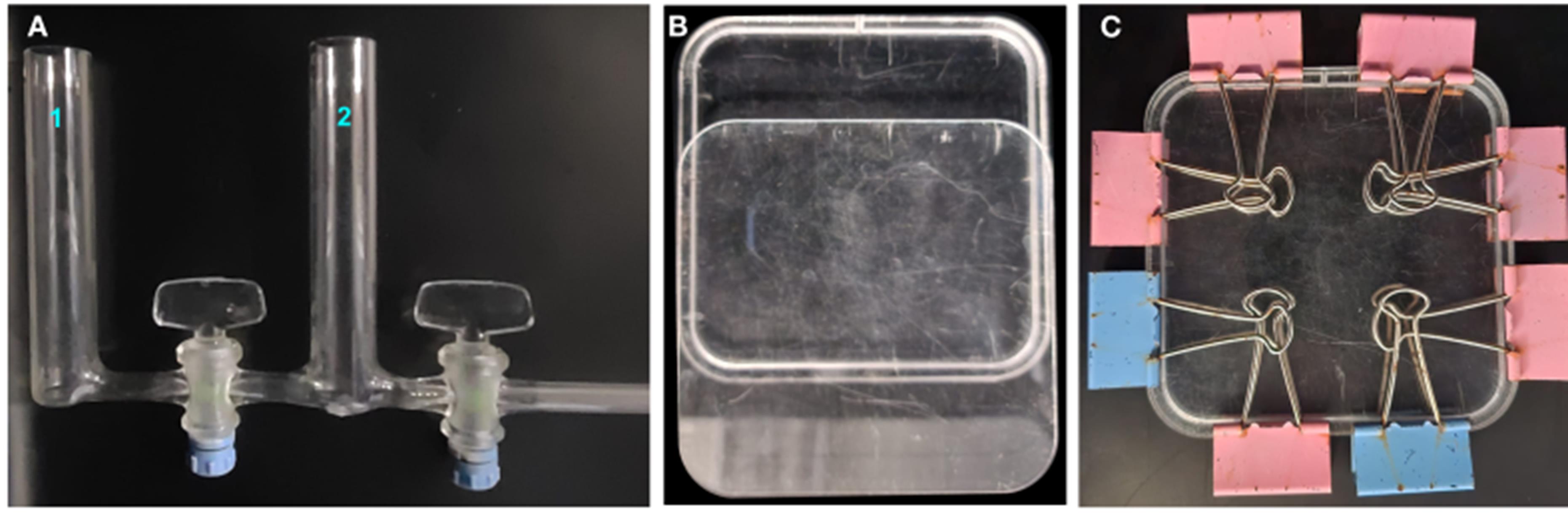
Figure 1. System components to create the osmotic gradient. (A) Gradient mixer. (B, C) Square acrylic vertical container.
2. Square acrylic vertical container with the exact dimensions of a Petri dish (120 mm width × 120 mm length × 5.7 mm depth, hole 2 mm diameter) (Figure 1B, C)
3. Square Petri dishes (120 × 120 mm) (Deltalab, catalog number: 200204)
4. 10 μL pipette tips (Tarsons, catalog number: 528100)
5. 20 μL pipette tips (Tarsons, catalog number: 528101)
6. 200 μL pipette tips (Tarsons, catalog number: 528104)
7. 1,000 μL pipette tips (Tarsons, catalog number: 528106)
8. MicroAmpTM Fast 8-tube strip, 0.1 mL (Applied Biosystems, catalog number: 4358293)
9. MicroAmpTM Optical 8-cap strips (Applied Biosystems, catalog number: 4323032)
10. Sterile 1.5 mL Eppendorf-like BIOLOGUX tubes (Biriden, catalog number:80-1500)
11. 4-way interlock flipper (SSIbio, catalog number: 5410-29)
12. Stacking 96-well PCR WorkUp rack and lead (SSIbio, catalog number: 5240-09)
13. Borosilicate glass media bottle, 500 mL, GL-45, blue caps, Schott (Droguería Paysandú)
14. Beakers borosilicate glass, 100, 200, 500, 1,000 mL (Droguería Paysandú)
15. Graduated cylinder borosilicate glass, 100, 500, 1,000 mL (Droguería Paysandú)
16. Pellet pestles (Sigma-Aldrich, catalog number: Z359963)
17. Autoclavable spatula (10 cm width)
18. PVC film (RolloPack)
19. Microscope slides and coverslips (CITOGLAS, Palmer Uruguay)
Equipment
1. Autoclave (DAIHAN Scientific, model: Fuzzy control 47Lit. MaXterile 47)
2. Horizontal laminar flow cabinet with UV lamp (Streamline® Laboratory products, Singapore)
3. Mr. FrostyTM freezing container (Thermo Fisher Scientific, catalog number: 5100-0001)
4. Liquid nitrogen (N2) tank model MVE XC20 (MVE Biological Solutions, catalog number:16520/2026)
5. Benchtop dewar flask (Thermo Fisher Scientific, catalog number: 4150-2000)
6. Freezer (-20 °C)
7. Refrigerator (2–8 °C)
8. Pipetman 4-Pipette kit, P2, P20, P200, P1000 (Gilson, catalog number: F167360)
9. Laboratory centrifuge model ST-8/8R (Thermo Fisher Scientific, catalog number: 75007204)
10. Rotor MicroClick 30×2 fixed angle microtube rotor for Sorvall ST8/ST8R (THERMO, catalog number: 75005719)
11. QuantStudioTM 5 Real-Time PCR System, 96-well, 0.1 mL (Applied Biosystems, Thermo Fisher Scientific, catalog number: A28138)
12. OACTONTM pH700 benchtop meter and stand (OACTON, catalog number: 35419-12)
13. Epifluorescence microscope, AXIO Imager, M2 with DIC (differential interference contrast) or Nomarski optics (ZEISS)
14. Digital camera (Sony, model: Cyber-shot DSC-HX1)
15. Controlled environmental chamber (PERCIVAL SCIENTIFIC, INC., USA)
16. Multifunction vortex mixer set VM-10 (DAHIAN®, catalog number: DH.WVM00020)
17. Pop-off cup head PM210 (DAHIAN®, catalog number: DH.WVM00210)
18. High-performance mini-microcentrifuge set CF-5, Class-I medical device (NIDS), Max. 5,500 rpm (DA DAIHAN®.WCF000, catalog number: DH.WCF00025) with circular fixed-angle rotor for 6× 0.2/0.5/1.5/2.0 mL tubes (DAIHAN®, catalog number: DH.WCF00105)
19. Nanodrop LITE (Thermo Scientific, catalog number: 840281500)
Software and datasets
1. ImageJ Fiji [8], free to use
2. R software [9], free to use
3. Zeiss ZENpro-Imaging Software, requires a license
4. Design and analysis software 2.7.0 QuantStudioTM (Applied Biosystems, Thermo Fisher Scientific), requires a license
5. InfoStat versión 2011 [10]
6. Excel Microsoft Corporation (2024) [11]
7. RT-qPCR results: ttl_col_dataset.xls (File S1)
8. Root growth rate data sets from osmotic gradient: data.RGR-G.xls (File S2); osmotic shock: data.RGR-S.xls (File S3)
Code
library(tidyverse)# Read datattl0 <- read_csv(file = 'ttl_col_dataset.csv', col_names = T) %>% mutate(Sample = paste(Genotype, Condition, sep = '_'))ttl_df <- ttl0 %>% dplyr::select(c(Sample, Gene, Log2FC, Rep, Condition, Genotype)) %>% pivot_wider(names_from = 'Gene', values_from = 'Log2FC')# Distances Heatmap -------------------------------------------------------library("pheatmap")ttl_mat <- ttl_df[,-c(1,2,3,4)] %>% as.matrix()rownames(ttl_mat) <- paste(rep(c('Col-0', 'ttl1'), each = 9), rep(rep(c('Control', 'Osmotic Shock', 'Osmotic Gradient'), each = 3), 2))# Distances Matrixdist_mat <- dist(ttl_mat)sampleDistMatrix <- as.matrix(dist_mat)colors <- colorRampPalette( rev(brewer.pal(9, "Blues")) )(255)# Plotpheatmap(sampleDistMatrix, clustering_method = 'complete', col=colors, # labels_row = T, show_colnames = F)# PCA ---------------------------------------------------------------------library(FactoMineR)library(factoextra)# Tidy data for prcompttl_pca <- ttl_df[, -c(1,2,3,4)]# Dimension reduction using PCAres.pca <- prcomp(ttl_pca, scale = TRUE)## Biplotfviz_pca_biplot(res.pca, title = '', axes = c(1,2), habillage = interaction(ttl_df$Condition, ttl_df$Genotype), addEllipses = T, ellipse.type = 'confidence', col.ind = ttl_df$Condition, label = 'var', pointshape = 19, mean.point = T)+ geom_point(aes( shape = ttl_df$Genotype), size = 2)+ scale_color_manual(name = 'Conditions', labels = rep(c('Control', 'Gradient', 'Shock'), times = 2), values = c(paleta, paleta))+ scale_fill_manual(name = 'Conditions', labels = rep(c('Control', 'Gradient', 'Shock'), times = 2), values = c(paleta, paleta))+ scale_shape_discrete(name = 'Genotype', labels = c('Col-0', 'TTL1'))+ theme_bw(base_family = 'Arial')+ theme( legend.position = "bottom", legend.box = 'horizontal', legend.title = element_text(size = 11), legend.text = element_text(size = 10), axis.text.x = element_text(size = 10), axis.text.y = element_text(size = 10), axis.title.x = element_text(size = 12), axis.title.y = element_text(size = 12))# Heatmap -----------------------------------------------------------------library(RColorBrewer)library(gplots)heatmap_df <-ttl0 %>% group_by(Sample, Gene) %>% summarise(mLfc = median(Log2FC)) %>% pivot_wider(names_from = 'Gene', values_from = 'mLfc')heatmap_mat <- heatmap_df[,-1] %>% as.matrix()rownames(heatmap_mat) <- heatmap_df %>% pull(Sample)# Matrix for plotmatPlot <- t(heatmap_mat)ComplexHeatmap::pheatmap(matPlot, color = redgreen(75), # color = redblue(75), scale = 'row', cluster_cols = F, cluster_rows = clust_plot, # clustering_distance_rows = clust_plot, clustering_method = 'complete', gaps_col = 3, cutree_rows = 4, column_names_side = 'top', angle_col = '45')# Packageslibrary (emmeans)library (lme4)library(tidyverse)#Read data RGR #data.RGR.G <- read_delim (file ="data.RGR.G.csv", col_names = TRUE, delim = ",", na = "NA")data.RGR.S <- read_delim (file ="data.RGR.S.csv",col_names = TRUE, delim = ",", na = "NA"# Data analysismod.RGR.G <- lm (RGR ~ genotype + medium + genotype * medium, data = data.RGR.G)anova (mod.RGR.G)em.RGR.G <- emmeans (mod.RGR.G, ~ genotype * medium)cr.em.RGR.G <- contrast (em.RGR.G, method = "pairwise")mod.RGR.S <- lm (RGR ~ genotype + medium + genotype * medium, data = data.RGR.S)anova (mod.RGR.S)em.RGR.S <- emmeans (mod.RGR.S, ~ genotype * medium)cr.em.RGR.S <- contrast (em.RGR.S, method = "pairwise")Procedure
A. Preparation of the osmotic gradient
1. To generate the osmotic gradient, use a gradient maker (Figure 1A) and a square vertical acrylic container (Figure 1B, C).
Caution: For now, work in the laminar flow hood.
Note: Autoclave the gradient maker before use. Sterilize the square vertical acrylic container with 70% ethanol for 20 min, dry it with sterile gauze, and expose it to germicidal UVC light for 15 min.
2. Fill tube 2 of the gradient maker with 25 mL of osmotic shock plant growth media.
Critical: Work with the media at a temperature above 40 °C to avoid pipe plugging.
3. Open the Teflon faucet of tube 2 to allow the media to pour into the vertical acrylic container up to 3 cm.
Note: Allow the media containing the osmotic gradient to solidify inside the vertical acrylic container at 4 °C for 35 min.
Critical: Clean the gradient mixer between the disposal of the different media with high-temperature water (over 40 °C).
4. Fill tube 1 of the gradient maker with 20 mL of basic plant growth media and tube 2 with 20 mL of osmotic shock plant growth media.
5. Open both Teflon faucets to allow the media to mix and pour into the vertical acrylic container up to 4.5 cm.
Notes:
1. This mixture produces increasing osmotic potentials ranging from 0 to -1.2 MPa.
2. Allow the media containing the osmotic gradient to solidify inside the vertical acrylic container at 4 °C for 35 min.
6. Fill tube 1 with 17 mL of basic plant growth media.
7. Open both Teflon faucets to allow the media to pour into the vertical acrylic container up to 2 cm.
Note: Allow the media containing the osmotic gradient to solidify inside the vertical acrylic container at 4 °C for 35 min.
8. Transfer the osmotic gradient media to the final sterile square Petri dish with a sterile spatula.
Note: If necessary, store the medium at 4 °C vertically for a week.
9. Plate 50 mL of basic plant growth media in a square Petri dish and allow it to solidify.
10. Plate 50 mL of osmotic shock media in a square Petri dish and allow it to solidify.
B. Seed sterilization and plating
1. Put Arabidopsis seeds of the selected genotypes for sterilization in a 1.5 mL microcentrifuge tube.
2. Add 1 mL of 70% ethanol to the tube containing the seeds. Vortex and incubate for 7 min. In a laminar flow hood, remove the sterilization solution.
Critical: Use a different tip for each genotype to avoid cross-contamination of the seeds.
3. Add 1 mL of 20% sodium hypochlorite with TWEEN® 20. Vortex and incubate for 7 min.
4. Remove the sterilization solution and wash with sterile Milli-Q water five times.
5. Saw seeds on the square Petri dish containing basic plant growth media.
6. Seal the Petri dishes with RolloPack and put the seeds at 4 °C for 48 h in darkness to stratify.
7. Put the sown Square Petri dishes vertically in a controlled environment chamber: long-day photoperiod of 16 h light/8 h darkness, light intensity of 50 μEm-2·s-1, temperature of 22 °C, and 60% relative humidity.
8. Transfer 5–6 seedlings, 7 days post-germination, to the square Petri dish containing the osmotic treatments.
Caution: For the osmotic gradient treatment, place the root tips at 0 mM mannitol at the entry point of the gradient.
9. Put the square Petri dishes vertically in a controlled environment chamber with a long-day photoperiod of 16 h light/8 h darkness, light intensity of 50 μEm-2·s-1, temperature of 22 °C, and 60% relative humidity; allow them to grow for the period of your interest.
Caution: Monitor the plates daily to remove any contamination that might arise.
Note: In [7], the period was 25 days.
C. Analysis of root growth rate
1. Photograph the seedlings growing in the osmotic gradient daily with a digital camera, using a tripod to ensure the pictures are always taken at the same distance.
2. Use the line equation shown in Figure 2 and Table 1 to determine the osmotic potential at each ruler point.
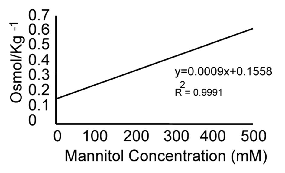
Figure 2. Estimating osmotic potential. The linear equation used to estimate the osmotic potential corresponding to each mannitol concentration is shown below the slope of the graph. The x-axis depicts the mannitol concentration in mM, and the y-axis depicts the solution's osmolality in Osmol/kg-1. The data used for the graphic representation are depicted in Table 1.
Table 1. Osmotic potentials measured using the cryoscopic osmometer model OSMOMAT 030 (Gonotech, Berlin, Germany).
| Mannitol concentration (mM) | Osmol/kg-1 | Osmotic potential (MPa) |
|---|---|---|
| 0 | 0.16 | -0.384 |
| 50 | 0.206 | -0.4944 |
| 100 | 0.248 | -0.5952 |
| 150 | 0.293 | -0.7032 |
| 200 | 0.336 | -0.8064 |
| 250 | 0.382 | -0.9168 |
| 300 | 0.425 | -1.02 |
| 350 | 0.474 | -11.376 |
| 400 | 0.522 | -12.528 |
| 450 | 0.572 | -13.728 |
| 500 | 0.624 | -14.976 |
3. Use a reference ruler that correlates the concentration of mannitol reached by the roots over time to the length of the vertical gradient (Figure 3B). The osmotic potential is derived from the calibration curves that correlate the concentration of mannitol with the osmotic potentials measured using the osmometer (Figure 2).
Note: Use the following formula to calculate the osmotic gradient to make the ruler: changes in concentration divided by the gradient length: Δ[mannitol] ÷ gradient length.
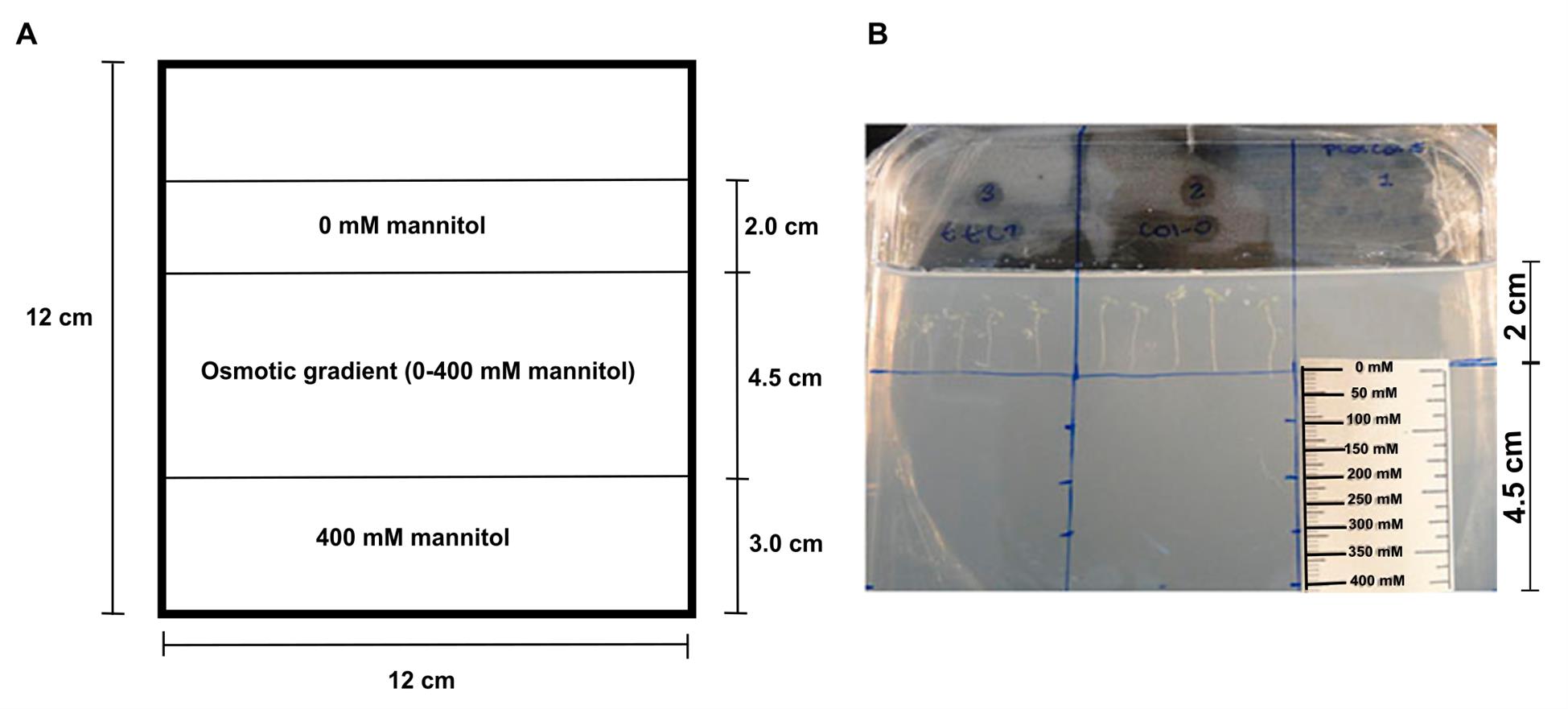
Figure 3. Representative scheme of a Petri dish containing the osmotic gradient. (A) Sequentially, 2 cm of basic plant growth media, 4.5 cm of osmotic gradient, and 3 cm of osmotic shock plant growth media. (B) Image depicting how seedlings were planted in the osmotic gradient system. Seedlings are placed in 0 mM mannitol, and the root tips are positioned at the entry to the gradient. The ruler used to obtain the mannitol concentration in the osmotic gradient reached by the root is shown.
4. Measure the root length from the hypocotyl to the tip using ImageJ Fiji's free software in each photograph [8] (Video 1).

5. Determine the root growth rate in a particular range of osmotic potential with the following formula: (root length reached at the highest osmotic potential – root length reached at the smallest osmotic potential/number of days).
D. Analysis of the proximal meristem
1. Clear the seedlings using Hoyer’s solution overnight at room temperature [12].
2. Cut the entire cleared root, mount on a microscope slide with 40 μL of Hoyer’s solution, and cover with the coverslip.
3. Photograph the microscopy preparation under a microscope with differential interference contrast (DIC).
4. Count cortex cells from the quiescence center to the first elongated cell in the photographs taken of the proximal meristem.
5. Measure cell length and width of cortex cells counted in step D4.
6. Measure the length and width of the mature cell.
Note: The first elongated cell is the start of the elongation zone, extending to the first root hair. The last cell of the elongation zone is considered the most elongated or mature cell [13].
7. Estimate growth parameters from cortical cell length as described before [14] for roots grown in the osmotic gradient.
a. Root growth rate:
b. Cell production rate:
c. Cell cycle length:
d. The average time interval between each cortical cell leaving the meristem to enter the TZ and EZ is 1/b.
E. Gene expression analysis
Below are the steps for preparing the differential gene expression experiment using RT-qPCR. The instructions are for three biological replicates, each containing 50–60 roots of seedlings grown for seven days under control and osmotic shock conditions (400 mM mannitol). For the osmotic gradient condition, each of the three replicas has 6–7 seedling roots grown for 25 days in the osmotic gradient condition when the proximal meristem of those roots reached the gradient in the range from 300 to 400 mM mannitol. Instances where the protocol can be interrupted/held are indicated by “pause point.”
1. RNA extraction
a. Extract RNA using TRIzolTM LS following the manufacturer’s instructions.
Critical: Use RNase-free tips with a filter and pipette. Once the RNA has been isolated, proceed to the cDNA synthesis, which is more stable than RNA.
b. Dissolve the RNA pellet in 20 μL of nuclease-free DEPC-treated water.
c. Save 1 μL of RNA for control.
d. Treat the RNA with 5 units of DNase I-RNase-free + 2 μL of 10× buffer.
e. Incubate at 37 °C for 10 min in a thermoblock.
f. Add 2 μL of 50 mM EDTA.
g. Heat-inactivate at 75 °C for 10 min.
Pause point: Store RNA at -80 °C (it could remain in this condition for several months).
h. Assess RNA integrity and quality by running an agarose gel electrophoresis (1%) in TAE 1× buffer.
2. cDNA synthesis
a. Estimate RNA integrity based on visualizing bands obtained in the agarose gels. Measure RNA concentration at 260 nm and purity using the 260/280 ratio using Nanodrop in order to proceed to the cDNA synthesis. A ratio of ~2.0 generally indicates pure RNA.
Note: Work at a lab bench or in a PCR cabinet after spraying with RNase AWAYTM reagent. Use RNase-free consumables and spray gloves with RNase AWAYTM reagent.
b. Combine the components shown in Table 2 in a PCR tube (1 × 20 μL) with the SuperScript® IV Reverse Transcription kit.
Note: From this point onward, there is no need to maintain RNase-free conditions. Work in the laminar flow hood.
Table 2. Retrotranscription reaction setup
| Reagent | Final concentration | Quantity or Volume |
|---|---|---|
| DEPC-treated water | n/a | up to 20 μL |
| 5× SSIV buffer | 1× | 4 μL |
| 10 mM dNTP mix (10 mM each) | 0.5 μM each | 1 μL |
| 100 mM DTT | 5 mM | 1 μL |
| RNase OUT RNase inhibitor (40 U/ μL) | 2 U/μL | 1 μL |
| 50 μM oligo d (T)20 primer | 2.5 μM | 1 μL |
| Template RNA | varies | <5 μg of total RNA or <500 ng of mRNA |
| SuperScript® IV reverse transcriptase (200 U/μL) | 10 U/μL | 1 μL |
| Total (optional) | n/a | 20 μL |
c. Briefly vortex and spin the reaction tube and place on ice.
d. Incubate the reaction mixture at 50–55 °C for 10 min.
e. Inactivate the reaction by incubating it at 80 °C for 10 min.
3. RT-qPCR
For an RT-qPCR run, use three biological and two technical replicas for each genotype (Col-0 and ttl1) in the three experimental conditions (control, osmotic shock, and osmotic gradient). Primers of Arabidopsis AT3G18780 ACTIN 2 and AT4G37830 CYTOCHROME C OXIDASE RELATED gene [15] were tested for housekeeping genes. Both genes presented the same threshold cycle. In [7], we used CYTOCHROME C OXIDASE RELATED as the housekeeping gene.
a. Prepare the following reaction in a PCR tube (1 × 10 μL) (Table 3).
Table 3. RT-qPCR reaction composition (1 reaction of 10 μL)
| Reagent | Final concentration | Quantity or Volume |
|---|---|---|
| PowerUpTM SYBRTM Green Master Mix (2×) | 1× | 5 μL |
| 10 μM forward primer | 0.6 μM | 0.6 μL |
| 10 μM reverse primer | 0.6 μM | 0.6 μL |
| cDNA | ≤ 500 ng | 1 μL |
| Nuclease-free water | n/a | 2.8 μL |
| Total (optional) | n/a | 10 μL |
b. Briefly vortex and spin the reaction tube and place it on ice.
c. Set up the QuantStudioTM 5 Real-Time PCR System as below and perform RT-qPCR (Table 4).
Table 4. Cycling program for RT-qPCR
| Steps | Temperature (°C) | Time | Cycles number |
| Activation UDG | 50 | 2 min | 1 |
| Initial denaturing | 95 | 2 min | 1 |
| Denature | 95 | 15 s | 40 |
| Annealing/extension | 60 | 1 min |
4. Calculation of primer’s efficiency: Calculating the efficiency of the primers for the genes of interest is necessary before conducting differential gene expression experiments.
a. Mix different cDNAs and prepare six serial 1/10 dilutions.
b. Set up 12 RT-qPCR reactions according to Table 3, corresponding to two technical replicates for each dilution.
c. Briefly vortex and spin the reaction tube and place it on ice.
d. Set up the QuantStudioTM 5 Real-Time PCR System as below and perform the RT-qPCR (Tables 4 and 5).
Table 5. Melting curve conditions used for RT-qPCR
| Step | Variation rate (°C/s) | Temperature (°C) | Time |
|---|---|---|---|
| 1 | 1.6 | 95 | 15 s |
| 2 | 1.6 | 60 | 1 min |
| 3 | 0.15 | 95 | 15 s |
e. After the run, extract the CT values of each sample and calculate the average of the technical replicates for each sample.
f. Plot a standard curve using the logarithms of the dilution values vs. the average CT values of the samples for each dilution. The expected result is a straight line with an R2 value close to 1, and the slope obtained from the equation of the line should be approximately -3.32, as this value assumes a primer efficiency of 100%. Once you determine the slope of the line, use the following equation:
Note: The calculated efficiency should range from 90% to 110%.
5. Cycle threshold (CT) adjustment of housekeeping gene
Before starting the differential gene expression assays, the CT adjustment of the housekeeping gene should be performed for all samples.
a. Run an RT-qPCR with the biological and technical replicates using primers for two housekeeping genes (AT3G18780: ACTIN 2 and AT4G37830: CYTOCHROME C OXIDASE-RELATED GENE [15]) of Arabidopsis.
b. Extract the CT values of all the samples from the run.
Note: The housekeeping gene must amplify at the same CT values across all samples (between 18 and 20); if not, cDNA concentration should be corrected using the following formula:
6. Fold-change calculations
Use the Livak method (2-ΔΔCT) [16] for the fold-change calculations or expression change rates of the different genes evaluated.
Note: If the efficiencies of the primer pairs used in a differential gene expression assay do not have similar and efficient amplification (between 90% and 110%), Pfaffl's mathematical adjustment [17] must be applied to calculate fold change.
In each qPCR run, primers for amplifying the housekeeping gene were included. The Col-0 control samples were used as the calibrator condition to normalize the ΔCT of the Col-0 samples under shock and osmotic gradient conditions, as well as the ttl1 samples under control, shock, and osmotic gradient conditions. Additionally, a negative control with no cDNA template was included in each experiment.
Note: The dissociation curves were used to indicate correct amplification.
Data analysis
Root growth rate data analysis was performed with a two-way ANOVA, followed by a mean comparison test using R software [9] to identify significant differences. Gene expression data analysis was performed with a two-way ANOVA using INFOSTAT [10] to evaluate genotype-by-environment interactions, applying a multiple testing correction with a significance threshold of p ≤ 0.05. Additionally, a one-way ANOVA in Excel [11] was used to assess differential gene expression among genotypes under control conditions (Supplemental Tables 4 and 5). Heatmap diagrams were generated using the 2-ΔΔCT method, assuming ideal amplification efficiency. Principal component analysis (PCA) and heatmap visualization were conducted using the FactoMineR [18] and pheatmap [19] packages in R [9], with gene expression values scaled across samples to highlight differences.
Validation of protocol
This protocol was validated by visual confirmation of gradient formation using Congo Red dye and a seed germination assay using Arabidopsis ttl1 mutant (known for its increased germination under osmotic stress conditions [20]) and its background line Col-0. A negative correlation was observed between the increased osmotic potential and the percentage of seed germination for both genotypes (correlation for Col-0: r = -0.92, p = 5.75281E-33; correlation for ttl1: r = -0.96, p = 2.69247E-45). Interestingly, at 400 mM of mannitol, the ttl1 mutant exhibited a 60% reduction in germination compared to an 80% reduction in Col-0 (Figure 4), in agreement with what was reported for ttl1 [20].
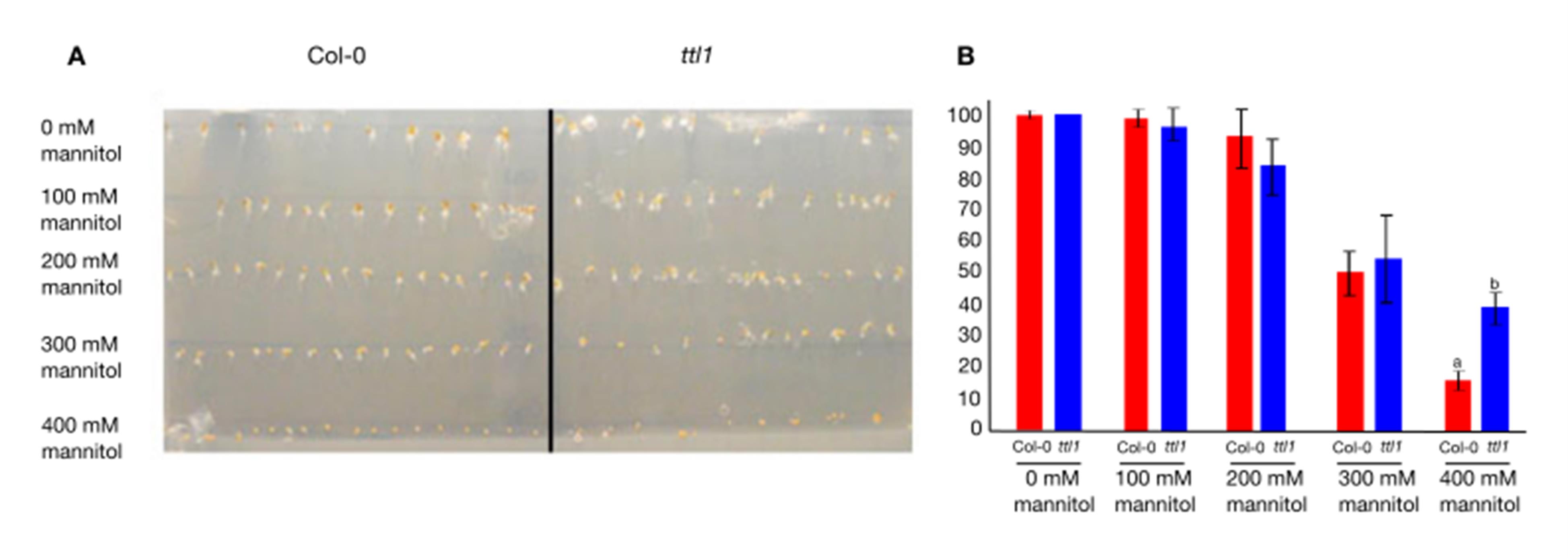
Figure 4. Seed germination assay for the validation of osmotic gradient system. (A) Seed germination assay installed in the osmotic gradient. (B) Germination percentage of Arabidopsis Col-0 and ttl1 seeds plated at different points of the osmotic gradient. The assay was repeated 4 times, with ≥19 seeds of each genotype placed in each mannitol concentration, as shown in (A). The letters indicate statistical differences (Student’s test, p value < 0.05).
This protocol has been used and validated in the following research article:
• Píriz-Pezzutto et al. [7]. Arabidopsis root apical meristem adaptation to an osmotic gradient condition: an integrated approach from cell expansion to gene expression. Front Plant Sci. 15: e1465219. https://doi.org/10.3389/fpls.2024.1465219 (Figure 1A, C; Figure 2A–C; Figure 3A–C; Figure 4, and Figure 5).
A dataset of RT-qPCR results (Files S1) and two root growth rate datasets (Files S2 and S3) are included in the Supplementary information, as well as the corresponding data analysis code used for validation.
General notes and troubleshooting
Troubleshooting
Problem 1:
The main problem that can occur is that we work in semi-sterile conditions because the vertical acrylic plates are not autoclavable. Even though they are sterilized with 70% ethanol for 20 min, dried with sterile gauze, and exposed to germicide UVC light for 15 min, and the osmotic gradient culture medium is prepared in a laminar flow hood using these acrylic plates and then transferred with the help of a sterile 10 cm wide spatula to the final sterile Petri dishes, sometimes contaminations might appear. For these reasons, the plates are monitored daily to remove any contamination, and it is recommended not to work for long periods of time.
Problem 2:
The tubing of the gradient mixer can be obstructed if the temperature of the agar media goes below 40 °C. To solve this problem, it is essential to work with the media in temperatures between 40 and 50 °C. Also, clean the tubes between different media with sterile water at 50 °C.
Supplementary information
The following supporting information can be downloaded here:
1. File S1. ttl_col_dataset.xls
2. File S2. data.RGR-G.xls
3. File S3. data.RGR-S.xls
Acknowledgments
Author contributions: S.P.-P.: Investigation, Methodology, Writing-Review & Editing. M.M.-M.: Formal Analysis. MMS: Writing-Review & editing. O.B.: Conceptualization, Funding acquisition. M.S.-S.: Conceptualization, Data curation, Investigation, Methodology, Supervision, Writing-Original Draft, Writing-review & editing. Funding sources that supported the work: ANII-FCE, grant No. 156503, and PEDECIBA. S.P.-P. and M.M.-M. received a fellowship from ANII and CAP, UdelaR. We thank Gastón Quero for root growth rate estimations. We thank Departamento de Biología Molecular y Bioquímica, Instituto de Hortifruticultura Subtropical y Mediterránea "La Mayora," Universidad de Málaga-Consejo Superior de Investigaciones Científicas (IHSM-UMA-CSIC), Universidad de Málaga, Campus Teatinos, 29071 Málaga, Spain, for the measurements done with the cryoscopic osmometer. This protocol was used in [7].
The following figures were created using BioRender: Graphical overview, Piriz, S. (2025) https://BioRender.com/yrzgznn; the cover image for the article: Piriz, S (2025) https://BioRender.com/jqxuhn7.
Competing interests
The authors declare no conflicts of interest.
References
- Gorgues, L., Li, X., Maurel, C., Martinière, A. and Nacry, P. (2022). Root osmotic sensing from local perception to systemic responses. Stress Biol. 2(1): 36. https://doi.org/10.1007/s44154-022-00054-1
- Rowe, J. H., Topping, J. F., Liu, J. and Lindsey, K. (2016). Abscisic acid regulates root growth under osmotic stress conditions via an interacting hormonal network with cytokinin, ethylene and auxin. New Phytol. 211(1): 225–239. https://doi.org/10.1111/nph.13882
- Cajero-Sanchez, W., Aceves-Garcia, P., Fernández-Marcos, M., Gutiérrez, C., Rosas, U., García-Ponce, B., Álvarez-Buylla, E. R., Sánchez, M. d. l. P. and Garay-Arroyo, A. (2019). Natural Root Cellular Variation in Responses to Osmotic Stress in Arabidopsis thaliana Accessions. Genes (Basel). 10(12): 983. https://doi.org/10.3390/genes10120983
- Yuan, T., Xiang, Z., Li, W., Gao, X. and Lu, Y. (2021). Osmotic stress represses root growth by modulating the transcriptional regulation of PIN‐FORMED3. New Phytol. 232(4): 1661–1673. https://doi.org/10.1111/nph.17687
- Cuadrado-Pedetti, M. B., Rauschert, I., Sainz, M. M., Amorim-Silva, V., Botella, M. A., Borsani, O. and Sotelo-Silveira, M. (2021). The Arabidopsis TETRATRICOPEPTIDE THIOREDOXIN-LIKE 1 Gene Is Involved in Anisotropic Root Growth during Osmotic Stress Adaptation. Genes (Basel). 12(2): 236. https://doi.org/10.3390/genes12020236
- Verslues, P. E., Agarwal, M., Katiyar‐Agarwal, S., Zhu, J. and Zhu, J. (2006). Methods and concepts in quantifying resistance to drought, salt and freezing, abiotic stresses that affect plant water status. Plant J. 45(4): 523–539. https://doi.org/10.1111/j.1365-313x.2005.02593.x
- Píriz-Pezzutto, S., Martínez-Moré, M., Sainz, M. M., Borsani, O. and Sotelo-Silveira, M. (2024). Arabidopsis root apical meristem adaptation to an osmotic gradient condition: an integrated approach from cell expansion to gene expression. Front Plant Sci. 15: e1465219. https://doi.org/10.3389/fpls.2024.1465219
- Schindelin, J., Arganda-Carreras, I., Frise, E., Kaynig, V., Longair, M., Pietzsch, T., Preibisch, S., Rueden, C., Saalfeld, S., Schmid, B., et al. (2012). Fiji: an open-source platform for biological-image analysis. Nat Methods. 9(7): 676–682. https://doi.org/10.1038/nmeth.2019
- R Core Team R. (2021). A Language and Environment for Statistical Computing.https://doi.org/10.32614/r.manuals
- Di Rienzo, J.A., C.F., B.M.G., G.L., T.M. and R.C.W. (2011). INFOSTAT.
- Excel Microsoft 365 Subscription 2024.
- Anderson, L. E. (1954). Hoyer's Solution as a Rapid Permanent Mounting Medium for Bryophytes. Bryologist. 57(3): 242–244. https://doi.org/10.1639/0007-2745(1954)57[242:hsaarp]2.0.co;2
- Perilli, S. and Sabatini, S. (2010). Analysis of Root Meristem Size Development. Methods Mol Biol. 655: 177–187. https://doi.org/10.1007/978-1-60761-765-5_12
- Cole, R. A., McInally, S. A. and Fowler, J. E. (2014). Developmentally distinct activities of the exocyst enable rapid cell elongation and determine meristem size during primary root growth in Arabidopsis. BMC Plant Biol. 14(1): e1186/s12870–014–0386–0. https://doi.org/10.1186/s12870-014-0386-0
- Geng, Y., Wu, R., Wee, C. W., Xie, F., Wei, X., Chan, P. M. Y., Tham, C., Duan, L. and Dinneny, J. R. (2013). A Spatio-Temporal Understanding of Growth Regulation during the Salt Stress Response in Arabidopsis. Plant Cell. 25(6): 2132–2154. https://doi.org/10.1105/tpc.113.112896
- Livak, K. J. and Schmittgen, T. D. (2001). Analysis of Relative Gene Expression Data Using Real-Time Quantitative PCR and the 2−ΔΔCT Method. Methods. 25(4): 402–408. https://doi.org/10.1006/meth.2001.1262
- Pfaffl, M. W. (2001). A new mathematical model for relative quantification in real-time RT-PCR. Nucleic Acids Res. 29(9): 45e–45. https://doi.org/10.1093/nar/29.9.e45
- Lê, S., Josse, J. and Husson, F. (2008). FactoMineR: AnRPackage for Multivariate Analysis. J Stat Softw. 25(1): ei01. https://doi.org/10.18637/jss.v025.i01
- Kolde, R. (2019). Pheatmap: pretty heatmaps. R package version, Vol. 726. https://doi.org/10.32614/cran.package.pheatmap
- Rosado, A., Schapire, A. L., Bressan, R. A., Harfouche, A. L., Hasegawa, P. M., Valpuesta, V. and Botella, M. A. (2006). The Arabidopsis Tetratricopeptide Repeat-Containing Protein TTL1 Is Required for Osmotic Stress Responses and Abscisic Acid Sensitivity. Plant Physiol. 142(3): 1113–1126. https://doi.org/10.1104/pp.106.085191
Article Information
Publication history
Received: Mar 31, 2025
Accepted: Jun 24, 2025
Available online: Jul 13, 2025
Published: Jul 20, 2025
Copyright
© 2025 The Author(s); This is an open access article under the CC BY-NC license (https://creativecommons.org/licenses/by-nc/4.0/).
How to cite
Píriz-Pezzutto, S., Martínez-Moré, M., Sainz, M. M., Borsani, O. and Sotelo-Silveira, M. (2025). Evaluating Arabidopsis Primary Root Growth in Response to Osmotic Stress Using an In Vitro Osmotic Gradient Experimental System. Bio-protocol 15(14): e5397. DOI: 10.21769/BioProtoc.5397.
Category
Plant Science > Plant physiology > Abiotic stress
Plant Science > Plant physiology > Plant growth
Bioinformatics and Computational Biology
Do you have any questions about this protocol?
Post your question to gather feedback from the community. We will also invite the authors of this article to respond.