- Protocols

- Articles and Issues
- For Authors
- About
- Become a Reviewer

Optimizing Confocal Imaging Protocols for Muscle Fiber Typing in the Mouse Masseter Muscle
Published: Vol 15, Iss 7, Apr 5, 2025 DOI: 10.21769/BioProtoc.5267 Views: 2948
Reviewed by: Sreejith PerinthottathilElena A. OstrakhovitchAnonymous reviewer(s)
Advertisement


Protocol Collections
Comprehensive collections of detailed, peer-reviewed protocols focusing on specific topics


Related protocols

Abstract
The masseter muscle, a key orofacial muscle, demonstrates unique anatomical and functional properties, including sexual dimorphism in myosin heavy chain (MyHC) expression and complex fiber architecture. Despite its importance in mastication and relevance to various disorders, phenotypic characterization of the masseter remains limited. Conventional fluorescence microscopy has been a cornerstone in muscle fiber typing, reliably identifying MyHC isoforms and measuring fiber cross-sectional areas. Building on this foundation, confocal microscopy offers complementary advantages, such as enhanced resolution, increased flexibility for multiplexing, and the ability to visualize complex structures in three dimensions. This study presents a detailed protocol for using confocal microscopy to achieve high-resolution imaging and molecular characterization of masseter muscle cryosections. By leveraging advanced technologies such as white light lasers and extended z-length imaging, this method ensures precise spectral separation, simultaneous multichannel fluorescence detection, and the ability to capture muscle architecture in three dimensions. The protocol includes tissue preparation, immunostaining for MyHC isoforms, and postprocessing for fiber segmentation and quantification. The imaging setup was optimized for minimizing signal bleed through, improving the signal-to-noise ratio, and enabling detailed visualization of muscle fibers and molecular markers. Image postprocessing allows for quantification of the cross-sectional area of individual fibers, nuclei location measurements, and identification of MyHC isoforms within each fiber. This confocal microscopy–based protocol provides similar resolution and contrast compared to conventional techniques, enabling robust multiplexed imaging and 3D reconstruction of muscle structures. These advantages make it a valuable tool for studying complex muscle architecture, offering broad applications in muscle physiology and pathology research.
Key features
• Enables high-resolution imaging of muscle fiber architecture, capturing detailed spatial relationships using extended z-length and advanced spectral separation techniques.
• Supports simultaneous detection of multiple molecular markers for robust muscle fiber typing and molecular localization.
• Allows for the generation of three-dimensional models to analyze muscle structures such as neuromuscular junctions, extracellular matrix, and mitochondrial organization.
• Adaptable to various skeletal muscles and species, providing valuable insights into muscle physiology, regeneration, and disease processes.
Keywords: Muscle fiber typingGraphical overview
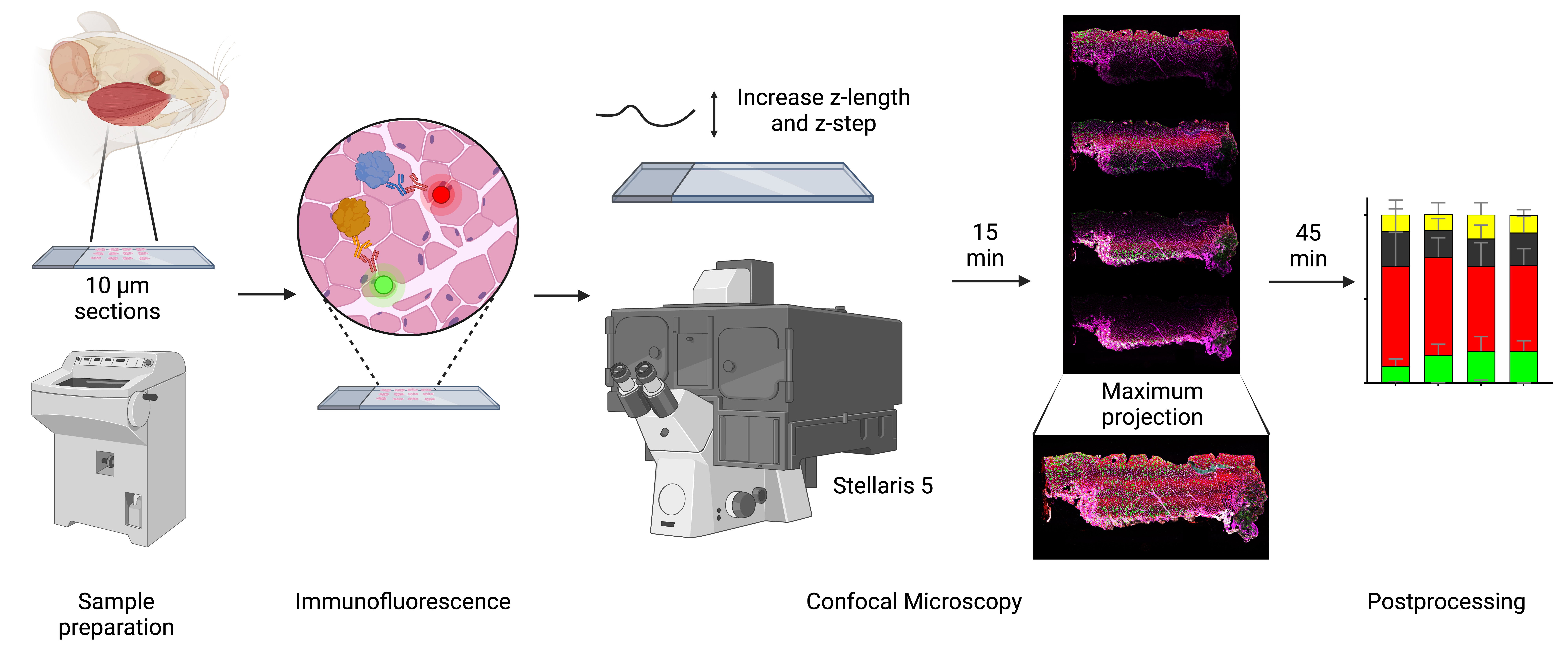
Analyzing muscle fiber composition and morphology in mice’s masseter muscle using confocal microscopy. Workflow for characterizing rodent masseter muscle fibers using advanced confocal microscopy. Confocal microscopy, equipped with white light laser technology and optimized z-stack imaging, allows precise spectral unmixing to reduce bleed through and enhance signal detection. The z-length is extended beyond the physical thickness of the sample to account for potential variations in tissue flatness and ensure complete imaging of all focal planes. The resulting high-resolution images provide detailed insights into fiber architecture, molecular composition, and cross-sectional areas, ensuring robust and reproducible data for analyzing the complex phenotypic characteristics of the masseter and other muscles.
Background
Skeletal muscles are heterogeneous, allowing them to engage in a spectrum of activities, from continuous low-intensity activity, such as breathing and posture control, to repeated submaximal or maximal contractions required for sprinting or lifting heavy objects [1]. Historically, muscle fibers have been categorized based on their morphological (red vs. white), biochemical (oxidative capacity, as determined by measuring succinate dehydrogenase, nicotinamide adenine dinucleotide dehydrogenase reductase, or ATP synthase activities), or molecular characteristics [2–6]. Currently, fiber types are distinguished based on the expression of specific myosin heavy chain (MyHC) isoforms. In adult rodent muscles, four major isoforms are detected, including type 1, 2A, 2X, and 2B (or a combination of these in hybrid fibers) corresponding to MYH7, MYH2, MYH1, and MYH4, respectively [1,3,7,8]. Type 1 fibers (slow twitch) have high mitochondrial content, oxidative metabolism, and slow contraction speed, making them well-suited for sustained endurance activities. Type 2A fibers (fast twitch oxidative) can generate greater power while maintaining endurance capacity. Type 2X and type 2B fibers (fast twitch glycolytic) contract the fastest and are adapted for short bursts of power. Noticeably, metabolic and contractile properties are highly adaptable and context-dependent, influenced by muscle function, species, and environmental factors rather than strictly by MyHC expression alone [3].
The orofacial muscles constitute a subset of skeletal muscle originating from the branchial arches, a distinct origin from muscles of the trunk and limbs [9]. The masseter is the dominant jaw-closing muscle in rodents, accounting for approximately 50% of the masticatory muscle mass and contributing to mastication, biting, and swallowing [10]. The adult muscle masseter consists of three anatomical partitions: superficial, intermediate, and deep [10–12]. Fiber orientation shifts from vertical in the anterior regions to an oblique orientation in the posterior aspect of the superficial and intermediate layers [10]. Notably, the insertion area for the superficial and deep masseter is vast, extending from the mandible angle to the first molar position for the superficial masseter and almost the entire length of the jugal bone for the deep masseter [10]. Given the complex architecture of the masseter, high-resolution imaging techniques are essential to capture its detailed structure [13]. However, the phenotypic characterization of the masseter remains limited [14,15].
Determining MyHC isoforms by immunofluorescence for muscle fiber typing has become widespread, in part because it also provides information about fiber cross-sectional areas [1,2,16]. Further, simultaneous labeling of muscle fibers is possible thanks to mouse monoclonal anti-MyHC antibodies with isotype-specific secondary antibodies [17]. Fluorescence microscopy often uses optical filters to separate emission from excitation light, accommodating several filter cubes, each one directing a specific predetermined wavelength [18]. Although only a single filter cube may be engaged at a time, there is potential for spectral overlap between fluorophores, limiting the number of compatible markers in a single experiment. Additionally, fluorescence microscopy captures light from all focal planes, limiting the signal-to-noise ratio and image resolution [19].
To overcome the limitations of widefield microscopy, Marvin Minsky developed the confocal microscope in 1957 [20]. Confocal microscopy provides better resolution than widefield fluorescent microscopes, yet its main advantage is the ability to acquire high-contrast images by minimizing out-of-focus light using a pinhole [18,21]. Additionally, confocal microscopy can capture multiple optical planes, making it ideal for analyzing compartmentalization and colocalization of specific molecules with high accuracy, as well as enabling the creation of 3D reconstruction of the imaged tissue [21]. Newer systems, such as the Stellaris 5 (Leica Microsystems, Durham, NC), feature next-generation white light lasers (WLL), which allow for the simultaneous excitation and detection of multiple fluorophores. The fine-tuning of excitation wavelengths enables highly efficient spectral unmixing, overcoming the limitations of traditional systems. This technology expands the range of usable fluorophores, including those in the near-infrared spectrum, and supports the use of multiple labels in parallel [22,23].
The objective of this study is to demonstrate the effective use of confocal microscopy in obtaining high-resolution, quantifiable images for muscle fiber typing from cryosections. We aim to show that this approach offers excellent resolution and contrast, even in applications where confocal capabilities are typically deemed unnecessary. Multiple fluorescent channels allow for the simultaneous visualization of several molecular markers in addition to the corresponding MyHC labels. This flexibility provides detailed insights into muscle fiber architecture and is particularly advantageous for reducing background noise and imaging alongside other protein targets that require precise 3D localization.
Materials and reagents
Biological materials
1. Adult female triple transgenic 3x-Tg-AD mice (Mutant Mouse Resource and Research Center, National Institutes of Health). Mice were 6–7 months old at tissue harvest. At 4 months of age, female 3xTg-AD mice show early signs of amyloid-beta plaques and tau phosphorylation, while behavioral phenotypes remain subtle and task-dependent [24–27]
2. Primary antibodies
a. Anti-laminin antibody (MilliporeSigma, catalog number: L9393, lot 0000234279, 0.5 mg/mL)
b. Anti-myosin heavy chain slow (Developmental Studies Hybridoma Bank–DSHB, catalog number: BA-F8, supernatant)
c. Anti-myosin heavy chain 2A (Developmental Studies Hybridoma Bank–DSHB, catalog number: SC-71, supernatant)
d. Anti-myosin heavy chain 2X (Developmental Studies Hybridoma Bank–DSHB, catalog number: 6H1, supernatant)
e. Anti-myosin heavy chain 2B (Developmental Studies Hybridoma Bank–DSHB, catalog number: BF-F3, supernatant)
3. Secondary antibodies
a. Goat anti-mouse IgG1 (Alexa FluorTM 488) (Thermo Fisher Scientific, catalog number: A-21121)
b. Goat anti-Mouse IgM heavy chain (Alexa FluorTM 546) (Thermo Fisher Scientific, catalog number: A-21045)
c. Goat anti-Mouse IgG2b (Alexa FluorTM 647) (Thermo Fisher Scientific, catalog number: A-21242)
d. Goat anti-Rabbit IgG (H+L) (Alexa FluorTM 750) (Thermo Fisher Scientific, catalog number: A-21039)
Reagents
1. 2-Methylbutane (Thermo Fisher Scientific, catalog number: 126470250)
2. Liquid nitrogen (Linde Gas & Equipment Inc, catalog number: NI 4.8LC23022SW)
3. Triton X-100 (MilliporeSigma, catalog number: T8787)
4. Normal goat serum (Thermo Fisher Scientific, catalog number: PCN5000)
5. Bovine serum albumin (BSA) (Equitech-Bio, catalog number: BAC62)
6. SlowFade Diamond antifade mountant (Thermo Fisher Scientific, catalog number: S36963)
7. Fisher Healthcare Tissue-PlusTM O.C.T. compound (Fisher Scientific, catalog number: 23-730-571)
8. Sodium chloride (NaCl) (MilliporeSigma, catalog number: S9625)
9. Potassium chloride (KCl) (MilliporeSigma, catalog number: P4504)
10. Sodium phosphate dibasic (Na2HPO4) (MilliporeSigma, catalog number: S0876)
11. Potassium phosphate monobasic (KH2PO4) (MilliporeSigma, catalog number: P5379)
12. 4',6-Diamidino-2-phenylindole dihydrochloride, 2-(4-Amidinophenyl)-6-indolecarbamidine dihydrochloride (DAPI) (Millipore Sigma, catalog number: D9542)
13. Dimethylformamide (MilliporeSigma, catalog number: 227056)
Solutions
1. Phosphate buffered saline (PBS) (see Recipes)
2. PBS + 0.1% Triton X-100 (see Recipes)
3. 0.5% BSA in 1× PBS (see Recipes)
4. Blocking solution (see Recipes)
5. Primary antibody solution (see Recipes)
6. Secondary antibody solution (see Recipes)
7. DAPI stock solution (see Recipes)
8. DAPI working solution (see Recipes)
Recipes
Note: Be precise about the ingredients (e.g., buffer or media), quantities, and conditions established for your experiments. Note that the omission of minor details from recipes (e.g., type of water used or storage conditions) might lead to the failure of the experiment.
1. Phosphate buffered saline (PBS) 1×
| Reagent | Final concentration | Quantity or Volume |
|---|---|---|
| NaCl | 137 mM | 8 g |
| KCl | 2.7 mM | 0.2 g |
| Na2HPO4 | 10 mM | 1.44 g |
| KH2PO4 | 1.8 mM | 0.245 g |
| Deionized water | n/a | to 1,000 mL |
2. PBS + 0.1% Triton X-100
| Reagent | Final concentration | Quantity or Volume |
|---|---|---|
| PBS 1× (Recipe 1) | 1× | 4.995 mL |
| Triton X-100 | 0.1% | 5 μL |
| Total | 5 mL |
3. 0.5% BSA in 1× PBS
| Reagent | Final concentration | Quantity or Volume |
|---|---|---|
| BSA | 0.5% | 250 mg |
| PBS 1× (Recipe 1) | 1× | to 50 mL |
Store at 4 °C for the duration of your experiment.
4. Blocking solution
| Reagent | Final concentration | Quantity or Volume |
|---|---|---|
| 0.5% BSA in 1× PBS (Recipe 3) | 1× | 315 μL |
| Normal goat serum | 10% | 35 μL |
Scale up when preparing multiple slides.
5. Primary antibody solution
| Reagent | Final concentration | Quantity or Volume |
|---|---|---|
| 0.5% BSA in 1× PBS (Recipe 3) | 1× | ~315 μL (per slide) |
| Normal goat serum | 2% | 7 μL |
| Primary antibody (four antibodies total) | 1:50 | 7 μL (per antibody per slide) |
Scale up when preparing multiple slides.
6. Secondary antibody solution
| Reagent | Final concentration | Quantity or Volume |
|---|---|---|
| 0.5% BSA in 1× PBS (Recipe 3) | 1× | ~315 μL (per slide) |
| Normal goat serum | 2% | 7 μL |
| Secondary antibody (four antibodies total) | 1:500 | 0.6 μL (per antibody per slide) |
Scale up when preparing multiple slides.
7. DAPI stock solution
| Reagent | Final concentration | Quantity or Volume |
|---|---|---|
| DAPI | 14.3 mM | 5 mg |
| Dimethylformamide | 12.87 M | 1 mL |
Mix to dissolve. It may take some time to completely dissolve. Protect from light, aliquot, and store at -20 °C.
8. DAPI working solution
| Reagent | Final concentration | Quantity or Volume |
|---|---|---|
| DAPI stock solution | 600 nM | 4 μL |
| PBS | 1× | 100 mL |
Store at 4 °C in a brown bottle or a bottle covered in foil. This should be stable for at least 6 months.
Laboratory supplies
1. VWR® Premium Superfrost® Plus microscope slides (VWR, catalog number: 48311-703)
2. VWR VistaVisionTM cover glasses, no. 1½ (VWR, catalog number: 16004-322)
3. ImmEdge® hydrophobic marker (Vector Laboratories, catalog number: NC9545623)
4. Coplin jar (Fisher Scientific, catalog number: E94)
5. Empty pipette tip box (Thermo Fisher Scientific, catalog number: 2069-05 or similar)
6. Paper towels (Kimberly-Clark ProfessionalTM, catalog number: 01804 or similar)
7. Dumont #7 curved forceps (Roboz, catalog number: RS-5047 or similar)
8. McPherson-Vannas curved spring micro scissors (Roboz, catalog number: RS-5631 or similar)
9. Cell lifters (Alkali Scientific, catalog number: TC7023 or similar)
10. Nail polish (Sally Hansen, catalog number: SALLYH2 or similar; avoid any glitter or metallic pigment colors)
Equipment
1. Leica CM1950 cryostat (Leica Biosystems, model: CM1950)
2. Confocal microscope (Leica Biosystems, model: Stellaris 5)
3. Wacom Intuos small Bluetooth tablet (Wacom, model: CTL4100WLK0)
Software and datasets
1. LAS X (Leica Biosystems)
2. FLIKA (version 0.3.1, free to use, available at https://flika-org.github.io/)
3. QuantiMus (free to use, available at https://quantimus.github.io/)
4. Image J (National Institutes of Health, version 1.54k, 15/10/2024)
Procedure
A. Sample preparation
1. Euthanize mice by CO2 followed by cervical dislocation and decapitation.
2. Immediately after euthanasia, excise the masseter muscle as follows [28,29]:
a. Make an incision along the lower jaw, carefully peel back the skin on the mouse’s face, and remove the parotid gland to expose the posterior part of the masseter muscle.
b. Using a pair of micro spring scissors, remove the fat and connective tissue around the muscle and detach the fascia covering the masseter.
c. Using forceps, dissect the masseter along its natural boundary, working from anterior to posterior tendon attachment, taking care not to damage muscle fibers.
d. Secure the anterior tendon using forceps and cut the tendon with a pair of scissors, while maintaining a grip with the forceps to prevent the muscle from retracting.
e. The deep and superficial masseters are closely attached to the surface of the mandible. Carefully pressing spring scissors against the mandible will ensure a complete dissection of the rest of the muscle.
Caution: Take care to distinguish the zygomaticomandibularis muscle, which is located along the zygomatic arch and the mandible. The masseter should be excised along its distinct boundaries to avoid contamination from neighboring muscles.
3. Once isolated, place the masseter muscle on a cell lifter, ensuring that it retains its proper shape and resting length.
4. Submerge the cell scraper holding the masseter in 2-methylbutane cooled to its freezing temperature in liquid nitrogen. Keep the muscle submerged for a minimum of 30 s to ensure thorough freezing.
Critical: Improper technique will lead to freezing artifacts and render the tissue inadequate for imaging and quantification.
5. Once frozen, transfer the muscle to a pre-cooled cryovial and store at -80 °C until further processing.
Pause point: Muscles can be stored at -80 °C for several months to years, provided the tissue remains undisturbed.
6. Mount the frozen tissue into the cryostat chuck using OCT and allow it to harden.
7. Section the muscle using a cryostat set to -20 °C.
8. Obtain serial sections of 10 μm, carefully placing them on the positively charged Superfrost® microscope slides. We collect four sections per muscle and up to six muscles per slide.
9. Allow the resulting slides to dry for at least 10 min to ensure proper tissue adhesion to the slides. Keep the slides at -20 °C until ready for immunofluorescence probing.
Pause point: Slides can typically be stored at -20 °C for a few weeks to several months.
B. Immunofluorescence
1. Allow the frozen slides to come to room temperature.
2. Create a hydrophobic barrier around the tissue sections using a hydrophobic marker to contain the staining reagents.
3. Permeabilize the tissue sections by incubating the slides with 400 μL of 0.1% Triton X-100 in 1× PBS (Recipe 2) for 2 min at room temperature. This volume of buffer is sufficient to cover 6 cm2 of the slide.
4. For blocking, incubate the slides in 10% goat serum and 0.5% BSA in 1× PBS (Recipe 4) at room temperature for 20 min to prevent nonspecific antibody binding. As in the previous step, 400 μL of blocking solution is sufficient to cover 6 cm2 or approximately one-third of the total area of the slide.
5. To probe with the primary antibody, dilute each antibody at 1:50 in a 0.5% BSA + 2% goat serum + 1× PBS solution (Recipe 5) and then incubate overnight in a humidified chamber at 4 °C. This chamber can be prepared by placing a wet paper towel inside an empty tip box, covered by the tip holder, which will hold the prepared slides.
Pause point: Allow the probing to occur for at least 8 h.
6. Wash the slides at room temperature for 5 min in a Coplin jar with enough PBS 1× (Recipe 1) to fill the jar. Repeat three times.
7. To probe with the secondary antibody, dilute each antibody at 1:500 in a 0.5% BSA + 2% goat serum + 1× PBS solution (Recipe 6) and then incubate at room temperature in the dark for 1 h.
Critical: Protect your slides from light for this and the following steps.
8. Wash the slides for 5 min in a Coplin jar with enough PBS 1× (Recipe 1) to fill the jar. Repeat three times.
9. Incubate each slide with 300 μL of DAPI working solution (Recipe 8) for 20 min.
10. Wash the slides for 5 min in a Coplin jar with enough PBS 1× (Recipe 1) to fill the jar. Repeat three times.
11. Add a drop of SlowFade Diamond antifade mountant and cover with a cover glass, avoiding any bubbles.
12. Seal the borders of the cover glass with nail polish and allow it to dry.
13. Once dry, move the slides to a storage box and keep at 4 °C until ready to image.
Caution/Pause point: Although the slides should be stable for a few weeks, all our slides were imaged within seven days of probing.
C. Confocal microscopy
1. Powering on your microscope system:
a. Locate the microscope control unit and switch the main power switch (upper switch) to the ON position.
b. Turn on the laser power switch (lower switch). Ensure the emission key is also on to enable laser activation.
2. Turn on the computer controlling the microscope and initiate the LAS X software. When prompted, select the option Machine to enable full microscope control.
Critical: Running the LAS X software in Simulation mode does not allow real-time visualization, scanning, or adjustment of microscope settings.
3. Open the sample stage, move the illuminator arm to the loading position, and securely place the microscope slide in the slide holder, ensuring proper alignment.
a. Once you have confirmed proper placement, return the illuminator arm to its original position and close the sample stage.
4. Using the touchscreen panel, select the 10× objective. Select the light path to go to the eyepiece and select the GFP channel for fluorescence visualization.
5. Locate your first region of interest by using the right lever of the joystick (located to the left of the microscope setup) to move the stage until you find the appropriate muscle section.
6. Adjust the focus using the left lever of the joystick until the image appears sharp through the eyepiece.
7. Once the section is in focus, disable the eyepiece visualization and return to the IF shutter mode to enable imaging via the confocal system.
8. Use the Leica LAS X Spectral Wizard for optimal channel setup according to the secondary antibodies used.
9. Use the 10× objective (HC PL APO 10×/0.40 CS2) and set the pinhole to 3.0 (Figure 1).
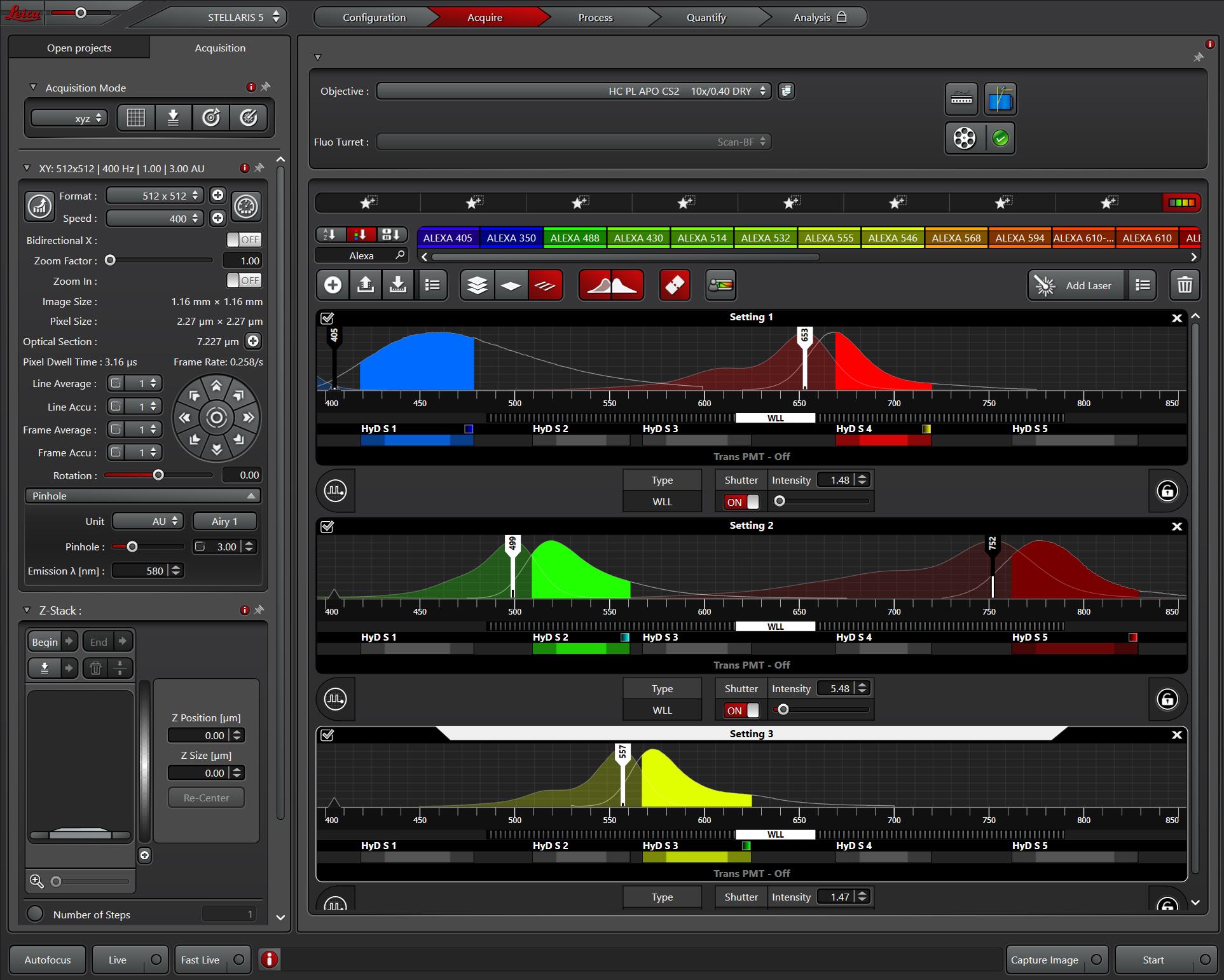
Figure 1. Microscope settings in LAS X for image acquisition. Settings for laser intensity, detection filters, and acquisition configurations are shown. Excitation and emission spectra for selected fluorophores (DAPI, Alexa FluorTM 488, Alexa FluorTM 546, Alexa FluorTM 647, and Alexa FluorTM 750) are displayed, with solid colors representing emission ranges and transparent overlays representing excitation ranges.
10. Increase the emission wavelengths for each fluorophore by 10 nm to ensure adequate separation between channels (Table 1).
Table 1. Selected emission range for secondary antibodies. Default emission ranges are set in the Leica LAS X software based on their spectral properties. Emission range modifications for selected fluorophores were implemented to reduce signal crosstalk between detection channels, enhancing specificity and improving data quality during multiplex confocal imaging on Stellaris 5.
| Antibody/fluorescent dye | Default excitation | Default emission range | Selected emission range |
|---|---|---|---|
| Goat anti-mouse IgG1 Alexa FluorTM 488 | 490 nm | 503–565 | 513–565 |
| Goat anti-mouse IgM (Heavy chain) Alexa FluorTM 546 | 557 nm | 557–625 | 567–625 |
| Goat anti-mouse IgG2b Alexa FluorTM 647 | 653 nm | 659–720 | 669–720 |
| Goat anti-rabbit IgG (H+L) Alexa FluorTM 750 | 752 nm | 752–795 | 762–795 |
11. Using the live imaging mode, adjust the intensities for each fluorescent channel manually based on signal-to-noise ratio optimization.
a. Click on the channel you wish to adjust and use the laser intensity knob to fine-tune each laser intensity, observing changes in the computer screen and adjusting as necessary.
b. On the upper-left side of the live image window, locate the image display mode button (which toggles between different visualization modes such as saturation, min/max scaling, and gamma). Use this button to determine the optimal intensity for each laser.
c. Switch to saturation mode to ensure that the intensity is not too high and adjust the laser intensity to optimize the signal-to-noise ratio without oversaturating the image.
d. Repeat this process for each laser wavelength.
12. Fine-tune the focus until the signal clarity is visually satisfactory across all channels.
13. In the Stage view, do a spiral scan to assess the positioning and overall area of the muscle to be scanned.
14. Scan the muscle at the optimal focal plane corresponding to the center of the muscle section. This will define the overall area of the muscle and identify any potential regions outside of the focus plane.
15. Any regions appearing out of focus on step C13 should be individually adjusted, and these focal adjustments should be used to set the z-length and z-steps.
16. For each muscle, we set the z-length at 20–60 μm and a z-step size between 5 and 10 μm. The total z-length and z-step intervals must be set to ensure that each potential muscle plane is captured at its optimal focal point.
a. The z-length was guided by the variability in focal planes observed during the preliminary scan in step C13, with greater variation (due to tissue folding or uneven adhesion) requiring a larger range.
b. Only the sharpest focal planes were selected for acquisition and maximum projection images, ensuring that out-of-focus regions were excluded.
17. Back in the Stage view, use the freehand drawing tool to outline the contour of the muscle to define the region of interest (ROI).
a. Once the selection is complete, the software automatically calculates and arranges the optimal number of tiles for scanning using the default overlap (10%), ensuring full coverage of the muscle while minimizing unnecessary overlap.
D. Postprocessing
1. Each imaged muscle consists of 15–25 panels, with the exact number determined by muscle size.
2. Use LAS X to perform the initial image stitching and deconvolution.
a. LAS X has built-in parameters for image stitching and deconvolution. Although it is possible to modify these parameters, we have not encountered any need to modify the default settings.
3. Select the maximum projections option to combine the different focal planes into a single image (Figure 2).
a. Click the Processing tab of LAS X and select the region to process.
b. Use the projection tab on the processing left panel, which will enable additional options in the bottom panel of the LAS X window.
c. Select Maximum from the projection list and preview the results. If you are satisfied with the image, click Apply, which will generate a processed image.
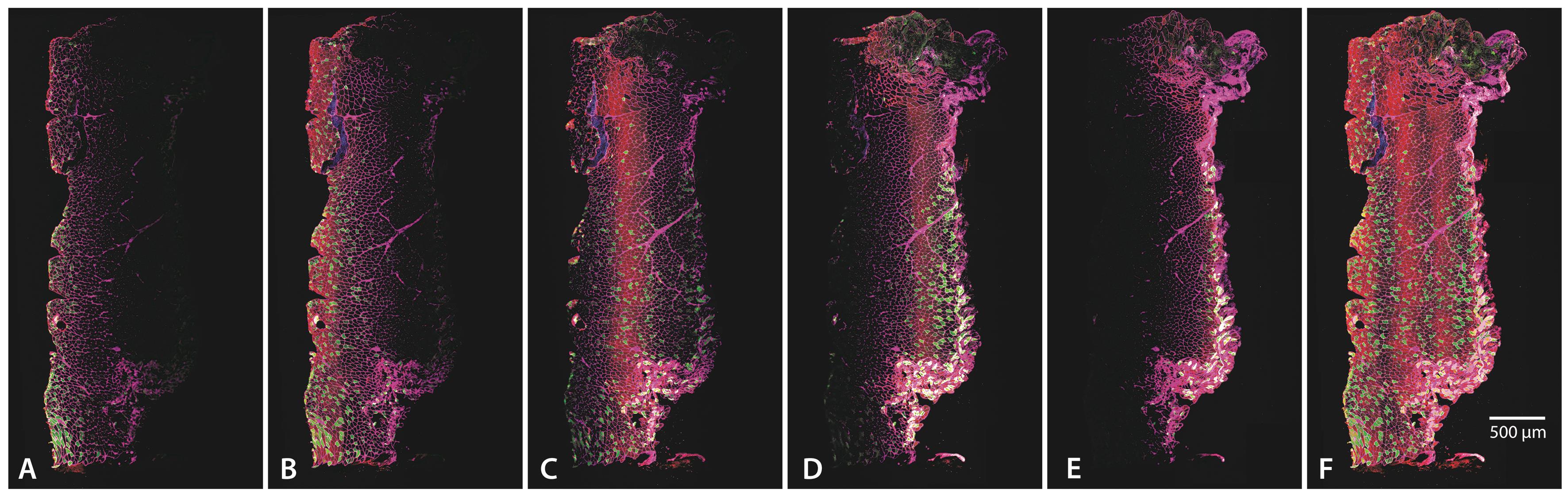
Figure 2. Individual focal planes and maximum projection. (A–E) The five different focal planes used for this specific section, all selected to account for uneven tissue adhesion to the slide. (F) Maximum projection, combining all focal planes to provide a comprehensive view of muscle architecture. Images were acquired using a 10× objective (HC PL APO 10×/0.40 CSA2). The scale bar represents 500 μm.
4. Export each individual channel for further processing and open each image in ImageJ. If the image was saved as a multichannel image, click Image > Color > Split channels to isolate and save the desired channel, discarding other channels in which there is no signal. Save the file with the appropriate identifier (i.e., name of the channel or primary antibody use) for easy identification and retrieval later.
5. If the laminin image shows any folding or tearing artifacts, trimming the image will facilitate accurate analysis. Using an Intuos drawing tablet, draw a mask containing all measurable fiber areas to remove any regions compromised by folding or tearing artifacts (Figure 3). This step may not be necessary for all muscles and can be achieved as follows:
a. Use the Freehand ROI tool and the drawing tablet to create the ROI in the laminin image that excludes the folding or tearing artifacts. After selecting the ROI, click Edit > Selection > Create Mask.
b. This action generates a new image where the outside of your selection is black and the selected area is white.
c. This mask can be saved, so you will not have to start from scratch if you need it again. However, the mask should be applied to individual channels, as the fiber typing software requires images of the same size for proper quantification, and applying the mask to a multichannel image will flatten all channels into RGB grayscale.
d. Apply the mask to the laminin by going to Process > Image Calculator. Image 1 is the mask, and image 2 is the laminin channel. Use “AND” for the operation, which will isolate the ROI in black background.
e. Save the resulting image as 8-bit with the appropriate qualifier (i.e., to distinguish between the cropped and the non-cropped image) (Figure 3).
f. Apply the mask to every individual channel corresponding to those of the myosin heavy chain antibodies and DAPI, as the fiber typing software requires all images from the same evaluated muscle to be the same size for accurate quantification. Save each resulting image as 8-bit with the appropriate qualifier.
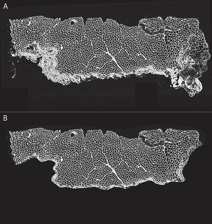
Figure 3. Image cropping to decrease artifacts. Using ImageJ and a Wacom drawing tablet, we created a mask to eliminate folded section areas, artifacts, or regions deemed non-analyzable. (A) Original and (B) cropped image.
6. Analyze the resulting 8-bit images using QuantiMus, a Flika plugin that allows for measuring the cross-sectional area (CSA), centrally nucleated fibers (CNF), and the fluorescence intensity of individual myofibers [30].
a. Open Flika and load the QuantiMus plugin.
b. Load the image corresponding to the laminin channel.
c. In the Fill Myofiber Gaps tab, select the laminin image. This will open a new window labeled Binary Markers.
d. Use the sliding thresholds to correct conjoined fibers and poorly distinguished boundaries. The blue threshold should be lower than the white. The default settings on QuantiMus have worked well for us. When the image is satisfactory, press Fill Myofiber Boundary Gaps, which will result in a new window labeled Binary Window.
e. Select the Define Myofibers tab and select the window corresponding to the binary window, which will generate a new window labeled Training image.
f. Select a few fibers and non-fibers by clicking once or twice. You need at least one of each, but we suggest you select several, even from different parts of the muscle, to encompass the variety in size and shape of myofibers. Additionally, you can filter the image by setting limits for size, circularity, etc. When several fibers have been selected, press Run Algorithm: Labeled Image.
g. You can manually select or deselect fibers as positive or negative or include more fibers in the training image and repeat the process until satisfied. Save the training data with a right-click on Save training data to use the same parameters to train other muscles within the same set.
h. Open one of the images containing a MyHC channel. Move to the Measure Fluorescence tab and select the trained and the single-channel images in their corresponding section. Press Measure Fluorescence, which will open a window of the single-channel image superimposed on the trained image.
i. Press Select Positives and, by adjusting the intensity slide bar, select some representative positive fibers (click to a yellow color), encompassing those with high and low intensity. Press Measure Positives to visualize (in blue) all fibers deemed “positive” for that specific myosin. Press Save Positives when all positive fibers have been categorized as such (Figure 4).
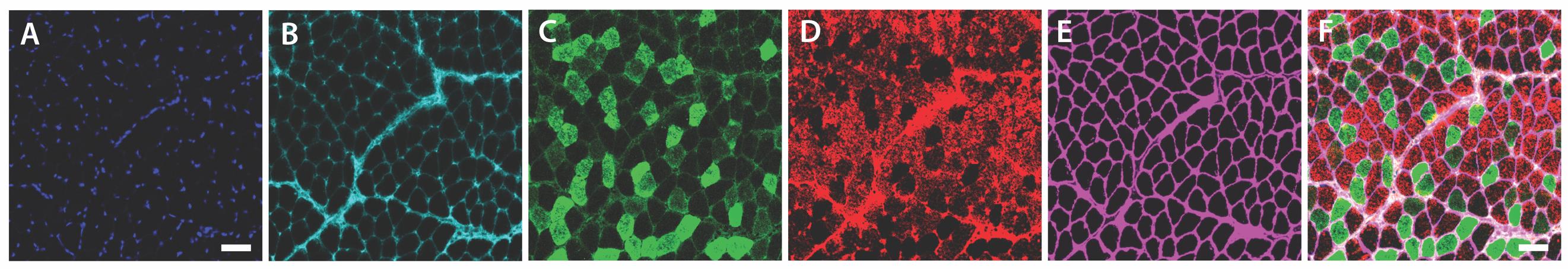
Figure 4. Representative fiber panel. Representative sections showing labeling for (A) nuclear stain (DAPI), (B) type 1 (MyHC 7, Alexa FluorTM 647), (C) type 2A (MyHC 2A, Alexa FluorTM 488), (D) type 2X (MyHC 1, Alexa FluorTM 546), and (E) Laminin (Alexa FluorTM 750). (F) Composite image with all channels merged, illustrating the overall fiber architecture. Unlabeled myofibers represent type 2B (MyHC 4) fibers. Scale bar represents 50 μm.
j. In the Print Data tab, select the correct pixels/micron ratio and press Print Data. This will generate an Excel file.
k. Repeat steps D6h–j for all other myosin channels.
l. If DAPI was used, go to the CNF tab to measure any potential centrally nucleated fibers. Open the image corresponding to the DAPI channel and select this and the trained image, creating a superimposed DAPI/trained fiber image.
Critical: The DAPI image must have been converted to a binary image for accurate nuclei identification. This can be achieved by opening the DAPI image on ImageJ, clicking Process > Binary > Make binary, and saving the resulting image.
m. Select the appropriate erosion for the myofibers, i.e., the region that is deemed acceptable for nuclei localization. The default option, 80, is appropriate for most muscles, but your needs may vary.
n. Measure the CNF and save the results. Print data to obtain an .xls file with your results.
7. Data analysis was performed on GraphPad Prism v 10.3.1.
Data analysis
Five wild-type mice were used as a pilot group, with each masseter muscle processed and analyzed separately. The average number of muscle fibers per masseter was 1,771. All fibers from the same masseter were included in the analysis, but individual fibers were not treated as replicates. Instead, each mouse represented a biological replicate, ensuring that data variability reflected inter-mouse differences rather than intra-sample variability. In our setup, antibodies against MYH1 (type 2X) and MYH4 (type 2B) share the same isotype (Mouse IgM), preventing their simultaneous use. Therefore, type 2B fibers were identified as unstained fibers in a slide probed for type 1, 2A, and 2X. If direct visualization of type 2B fibers is required, an alternative approach will include a separate slide probed with antibodies against type 1, 2A, and 2B MyHC.
Frequency distribution analysis (Figure 5) was performed by pooling the cross-sectional area (CSA) of all measured fibers. Statistical analysis was performed using GraphPad Prism. Data inclusion criteria required fibers to be intact and free of artifacts, such as folding or tearing. Longitudinal fibers were excluded from the analysis to prevent artificially large CSA values.
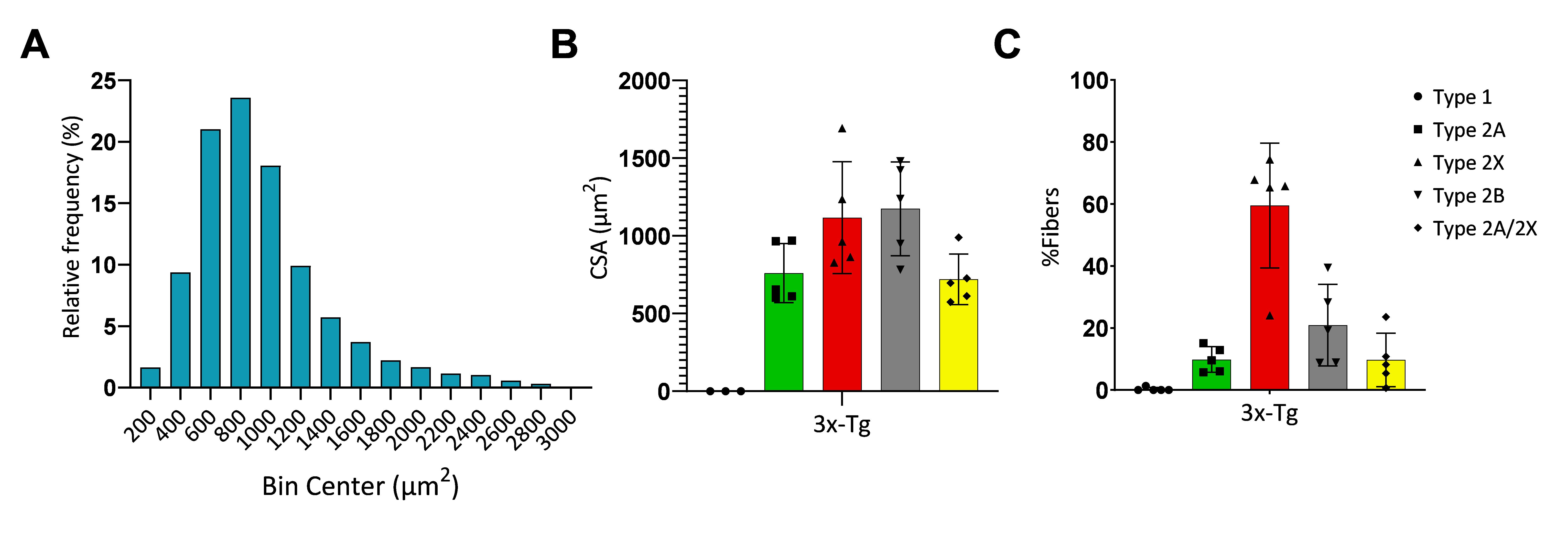
Figure 5. Cross-sectional area and myosin composition in masseter muscles. (A) Histogram for fiber distribution of the cross-sectional areas (CSA) in 3x-Tg mice. (B) Average fiber CSA for each myosin heavy chain (MyHC) isoform in 3x-Tg mice. (C) Relative proportions of MyHC (type 1, 2A, 2X, and 2B fibers). Type 2B fibers were calculated from non-stained fibers after probing, and type 2A/2X fibers were calculated from fibers that were positive for both type 2A and 2X MyHC. (n = 5, error bars represent SD.)
Validation of protocol
Although data on the phenotypic characteristics of the masseter is limited, the results obtained using this protocol align with previously published studies. In particular, the presence of type 2X fibers is consistent with the finding of Widmer et al., where these accounted for 50% of the total fibers in the masseter and were identified as fibers not stained by either 2A or 2B antibodies [11]. Other studies have highlighted a heterogeneous pattern of distribution, with specific fiber types clustering within the superficial or deep regions of the masseter [11,31,32]. Additionally, studies in rodents confirm the lack of type 1 fibers, and reiterate the predominance of type 2A, 2B, and 2X fibers [31,33].
Hybrid fibers, particularly 2A/2X and 2X/2B types, are a prominent feature of the masseter, as highlighted by Sano et al. and Monemi et al. [33,34]. These hybrid fibers further validate the protocol by demonstrating its capacity to capture the transitional properties of muscle fibers, which contribute to the functional versatility of the muscle.
Moreover, the CSA values reported in the aforementioned studies are consistent with those obtained using this protocol, with type 2B fibers exhibiting the largest CSA, followed by 2X and 2A fibers [11,12,31,32]. Collectively, these comparisons validate the robustness of the protocol in capturing physiologically relevant data on the heterogeneity and functional specialization of masseter muscle fibers.
General notes and troubleshooting
General notes
1. The antibodies used in this protocol enable the identification of multiple MyHC isoforms. However, some antibodies are the same isotype and cannot be used simultaneously under standard conditions. To address this limitation, emerging technologies now allow for the customization of fluorescent probes that conjugate directly to primary antibodies. These technologies enable researchers to bypass epitope compatibility issues and expand the number of fluorophores that can be used in a single experiment, significantly enhancing multiplexing capabilities.
2. Newer systems, such as the Stellaris 5 (Leica Microsystems, Durham, NC), feature next-generation white light lasers (WLL), which allow for the simultaneous excitation and detection of multiple fluorophores. The fine-tuning of excitation wavelengths enables highly efficient spectral unmixing, overcoming the limitations of traditional systems. This technology expands the range of usable fluorophores, including those in the near-infrared spectrum, and supports the use of multiple labels in parallel [22,23].
3. While the protocol was developed for the masseter muscle of mice, this approach offers robust, quantifiable data, supporting the effective use of confocal microscopy to study complex muscle structures, with a methodology adaptable to other muscle groups and species.
4. The confocal microscope’s ability to capture multiple optical planes and generate 3D reconstructions further improves the understanding of muscle fiber architecture and molecular localization. While fiber typing itself does not require 3D reconstruction, the same sections could be used to examine additional markers that benefit from precise cellular localization [35]. For example, with the proper markers, 3D imaging can reveal the spatial arrangement of mitochondria within muscle fibers, allowing for detailed analysis of mitochondrial density, volume, and distribution across different fiber types [36]. Additionally, 3D reconstruction is advantageous for visualizing neuromuscular junctions, capillary networks, and the extracellular matrix, which play critical roles in muscle function and are challenging to capture fully in 2D [37–39]. Examining these structures in 3D provides insights into how muscle fibers interact with their surrounding environment, including vascular and neural components, which are essential for understanding muscle health, regeneration, and disease.
Troubleshooting
Problem 1: Certain areas of the muscle are not visualized at a specific focal plane.
Possible cause: Variability can arise from differences in tissue preparation, section thickness, or adherence to the slide.
Solution: Extending the z-length during imaging can mitigate issues caused by uneven tissue flatness, ensuring all regions of interest are captured.
Problem 2: Myofibers exhibit a vacuolated or hollow appearance, resembling a donut-like structure.
Possible cause: Improper freezing technique, likely due to slow freezing or residual impurities in the freezing medium.
Solution: Ensure proper adherence to freezing instructions. Always use fresh 2-methylbutane and discard any leftover solution to prevent contamination or reduced freezing efficacy.
Problem 3: Fluorescent staining for laminin or a specific MyHC is weak or absent.
Possible cause: Primary or secondary antibodies degraded due to improper or very long storage duration.
Solution: Follow recommended storage conditions and purchase new antibodies if necessary.
Acknowledgments
Imaging was done at the Imaging Core, supported by the Indiana Center for Musculoskeletal Health. This work was supported by NIH (R01AG064003 and K02AG068595), VA Merit Pilot Award (I21BX006307), and the Hevolution foundation grant HF-GRO-23-1199172-46 (AM).
Competing interests
The authors declare no conflicts of interest.
Ethical considerations
All animal handling, housing, and procedures were approved by the Indiana University School of Medicine IACUC (Protocol 22036) and in accordance with ARRIVE guidelines [40].
References
- Schiaffino, S. and Reggiani, C. (2011). Fiber Types in Mammalian Skeletal Muscles. Physiol Rev. 91(4): 1447–1531. https://doi.org/10.1152/physrev.00031.2010
- Sawano, S. and Mizunoya, W. (2022). History and development of staining methods for skeletal muscle fiber types. Histol Histopathol. 37(6): 493–503. https://doi.org/10.14670/hh-18-422
- Blemker, S. S., Brooks, S. V., Esser, K. A. and Saul, K. R. (2024). Fiber-type traps: revisiting common misconceptions about skeletal muscle fiber types with application to motor control, biomechanics, physiology, and biology. J Appl Physiol. 136(1): 109–121. https://doi.org/10.1152/japplphysiol.00337.2023
- Cherian, K. M., Vallyathan, N. V. and George, J. C. (1965). Succinic dehydrogenase in pigeon pectoralis during disuse atrophy. J Histochem Cytochem. 13(4): 265–269. https://doi.org/10.1177/13.4.265
- Umeda, T., Kagawa, S. and Kawakatsu, K. (1965). Histochemical Observations of Succinic Dehydrogenase Activity in Facial Muscles of Mammalians. J Dent Res. 44(4): 815–820. https://doi.org/10.1177/00220345650440043001
- Novikoff, A. B., Shin, W. Y. and Drucker, J. (1961). Mitochondrial localization of oxidative enzymes: staining results with two tetrazolium salts. J Cell Biol. 9(1): 47–61. https://doi.org/10.1083/jcb.9.1.47
- Schiaffino, S., Saggin, L., Viel, A., Ausoni, S., Sartore, S. and Gorza, L. (1986). Muscle fiber types identified by monoclonal antibodies to myosin heavy chain. In: Biochemical Aspects of Physical Exercise. Elsevier Science Publishers, 27–34.
- Termin, A., Staron, R. S. and Pette, D. (1989). Myosin heavy chain isoforms in histochemically defined fiber types of rat muscle. Histochemistry. 92(6): 453–457. https://doi.org/10.1007/BF00524756
- Ono, Y., Boldrin, L., Knopp, P., Morgan, J. E. and Zammit, P. S. (2010). Muscle satellite cells are a functionally heterogeneous population in both somite-derived and branchiomeric muscles. Dev Biol. 337(1): 29–41. https://doi.org/10.1016/j.ydbio.2009.10.005
- Baverstock, H., Jeffery, N. S. and Cobb, S. N. (2013). The morphology of the mouse masticatory musculature. J Anat. 223(1): 46–60. https://doi.org/10.1111/joa.12059
- Widmer, C., Morris-Wiman, J. and Nekula, C. (2002). Spatial Distribution of Myosin Heavy-chain Isoforms in Mouse Masseter. J Dent Res. 81(1): 33–38. https://doi.org/10.1177/154405910208100108
- Widmer, C., English, A. and Morris-Wiman, J. (2007). Developmental and functional considerations of masseter muscle partitioning. Arch Oral Biol. 52(4): 305–308. https://doi.org/10.1016/j.archoralbio.2006.09.015
- Kupczik, K., Stark, H., Mundry, R., Neininger, F. T., Heidlauf, T. and Röhrle, O. (2015). Reconstruction of muscle fascicle architecture from iodine-enhanced microCT images: A combined texture mapping and streamline approach. J Theor Biol. 382: 34–43. https://doi.org/10.1016/j.jtbi.2015.06.034
- Yoshimi, T., Koga, Y., Nakamura, A., Fujishita, A., Kohara, H., Moriuchi, E., Yoshimi, K., Tsai, C. and Yoshida, N. (2017). Mechanism of motor coordination of masseter and temporalis muscles for increased masticatory efficiency in mice. J Oral Rehabil. 44(5): 363–374. https://doi.org/10.1111/joor.12491
- Moriuchi, E., Hamanaka, R., Koga, Y., Fujishita, A., Yoshimi, T., Yasuda, G., Kohara, H. and Yoshida, N. (2019). Development and evaluation of a jaw-tracking system for mice: reconstruction of three-dimensional movement trajectories on an arbitrary point on the mandible. BioMed Eng Online. 18(1): 59. https://doi.org/10.1186/s12938-019-0672-z
- Wang, C., Yue, F. and Kuang, S. (2017). Muscle Histology Characterization Using H&E Staining and Muscle Fiber Type Classification Using Immunofluorescence Staining. Bio Protoc. 7(10): e2279. https://doi.org/10.21769/bioprotoc.2279
- Sawano, S., Komiya, Y., Ichitsubo, R., Ohkawa, Y., Nakamura, M., Tatsumi, R., Ikeuchi, Y. and Mizunoya, W. (2016). A One-Step Immunostaining Method to Visualize Rodent Muscle Fiber Type within a Single Specimen. PLoS One 11(11): e0166080. https://doi.org/10.1371/journal.pone.0166080
- Sanderson, M. J., Smith, I., Parker, I. and Bootman, M. D. (2014). Fluorescence Microscopy. Cold Spring Harb Protoc. 2014(10): pdb.top071795. https://doi.org/10.1101/pdb.top071795
- Combs, C. A. and Shroff, H. (2017). Fluorescence Microscopy: A Concise Guide to Current Imaging Methods. Curr Protoc Neurosci. 79(1): e29. https://doi.org/10.1002/cpns.29
- Patil-Takbhate, B., Takbhate, R., Khopkar-Kale, P. and Tripathy, S. (2024). Marvin Minsky: The Visionary Behind the Confocal Microscope and the Father of Artificial Intelligence. Cureus. 16(9): e68434. https://doi.org/10.7759/cureus.68434
- Jonkman, J., Brown, C. M., Wright, G. D., Anderson, K. I. and North, A. J. (2020). Tutorial: guidance for quantitative confocal microscopy. Nat Protoc. 15(5): 1585–1611. https://doi.org/10.1038/s41596-020-0313-9
- Calvo, L., Ronshaugen, M. and Pettini, T. (2021). smiFISH and embryo segmentation for single-cell multi-gene RNA quantification in arthropods. Commun Biol. 4(1): 352. https://doi.org/10.1038/s42003-021-01803-0
- Jonkman, J. and Brown, C. M. (2015). Any Way You Slice It—A Comparison of Confocal Microscopy Techniques. J Biomol Tech. 26(2): 54–65. https://doi.org/10.7171/jbt.15-2602-003
- Yamada, C., Ho, A., Garcia, C., Oblak, A. L., Bissel, S., Porosencova, T., Porosencov, E., Uncuta, D., Ngala, B., Shepilov, D., et al. (2024). Dementia exacerbates periodontal bone loss in females. J Periodontal Res 59(3): 512–520. https://doi.org/10.1111/jre.13227
- Javonillo, D. I., Tran, K. M., Phan, J., Hingco, E., Kramár, E. A., da Cunha, C., Forner, S., Kawauchi, S., Milinkeviciute, G., Gomez-Arboledas, A., et al. (2021). Systematic Phenotyping and Characterization of the 3xTg-AD Mouse Model of Alzheimer's Disease. Front Neurosci. 15: 785276. https://doi.org/10.3389/fnins.2021.785276
- Billings, L. M., Oddo, S., Green, K. N., McGaugh, J. L. and LaFerla, F. M. (2005). Intraneuronal Abeta causes the onset of early Alzheimer's disease-related cognitive deficits in transgenic mice. Neuron. 45(5): 675–688. https://doi.org/10.1016/j.neuron.2005.01.040
- Belfiore, R., Rodin, A., Ferreira, E., Velazquez, R., Branca, C., Caccamo, A. and Oddo, S. (2019). Temporal and regional progression of Alzheimer's disease-like pathology in 3xTg-AD mice. Aging Cell. 18(1): e12873. https://doi.org/10.1111/acel.12873
- Carvajal Monroy, P. L., Yablonka-Reuveni, Z., Grefte, S., Kuijpers-Jagtman, A. M., Wagener, F. A. and Von den Hoff, J. W. (2015). Isolation and Characterization of Satellite Cells from Rat Head Branchiomeric Muscles. J Visualized Exp. e3791/52802. https://doi.org/10.3791/52802
- Cheng, X., Huang, Y., Li, Y., Li, J. and Wang, Y. (2023). Freezing Injury in Mouse Masseter Muscle to Establish an Orofacial Muscle Fibrosis Model. J Visualized Exp. e3791/65847. https://doi.org/10.3791/65847
- Kastenschmidt, J. M., Ellefsen, K. L., Mannaa, A. H., Giebel, J. J., Yahia, R., Ayer, R. E., Pham, P., Rios, R., Vetrone, S. A., Mozaffar, T., et al. (2019). QuantiMus: A Machine Learning-Based Approach for High Precision Analysis of Skeletal Muscle Morphology. Front Physiol. 10: e01416. https://doi.org/10.3389/fphys.2019.01416
- Eason, J. M., Schwartz, G. A., Pavlath, G. K. and English, A. W. (2000). Sexually dimorphic expression of myosin heavy chains in the adult mouse masseter. J Appl Physiol. 89(1): 251–258. https://doi.org/10.1152/jappl.2000.89.1.251
- Sciote, J. J., Horton, M. J., Rowlerson, A. M., Ferri, J., Close, J. M. and Raoul, G. (2012). Human Masseter Muscle Fiber Type Properties, Skeletal Malocclusions, and Muscle Growth Factor Expression. J Oral Maxillofac Surg. 70(2): 440–448. https://doi.org/10.1016/j.joms.2011.04.007
- Sano, R., Tanaka, E., Korfage, J. A., Langenbach, G. E., Kawai, N., van Eijden, T. M. and Tanne, K. (2007). Heterogeneity of fiber characteristics in the rat masseter and digastric muscles. J Anat. 211(4): 464–470. https://doi.org/10.1111/j.1469-7580.2007.00783.x
- Monemi, M., Eriksson, P. O., Kadi, F., Butler-Browne, G. S. and Thornell, L. E. (1999). Opposite changes in myosin heavy chain composition of human masseter and biceps brachii muscles during aging. J Muscle Res Cell Motil. 20(4): 351–361. https://doi.org/10.1023/A:1005421604314
- Luther, P. K. (2009). The vertebrate muscle Z-disc: sarcomere anchor for structure and signalling. J Muscle Res Cell Motil. 30(5–6): 171–185. https://doi.org/10.1007/s10974-009-9189-6
- Glancy, B., Hartnell, L. M., Malide, D., Yu, Z.-X., Combs, C. A., Connelly, P. S., Subramaniam, S. and Balaban, R. S. (2015). Mitochondrial reticulum for cellular energy distribution in muscle. Nature. 523(7562): 617–620. https://doi.org/10.1038/nature14614
- Egginton, S. and Gaffney, E. (2010). Tissue capillary supply--it's quality not quantity that counts! Exp Physiol. 95(10): 971–979. https://doi.org/10.1113/expphysiol.2010.053421
- Gillies, A. R. and Lieber, R. L. (2011). Structure and function of the skeletal muscle extracellular matrix. Muscle Nerve. 44(3): 318–331. https://doi.org/https://doi.org/10.1002/mus.22094
- Jones, R. A., Harrison, C., Eaton, S. L., Llavero Hurtado, M., Graham, L. C., Alkhammash, L., Oladiran, O. A., Gale, A., Lamont, D. J., Simpson, H., et al. (2017). Cellular and Molecular Anatomy of the Human Neuromuscular Junction. Cell Rep. 21(9): 2348–2356. https://doi.org/10.1016/j.celrep.2017.11.008
- Kilkenny, C., Browne, W. J., Cuthill, I. C., Emerson, M. and Altman, D. G. (2010). Improving Bioscience Research Reporting: The ARRIVE Guidelines for Reporting Animal Research. PLOS Biol. 8(6): e1000412. https://doi.org/10.1371/journal.pbio.1000412
Article Information
Publication history
Received: Dec 17, 2024
Accepted: Mar 3, 2025
Available online: Mar 20, 2025
Published: Apr 5, 2025
Copyright
© 2025 The Author(s); This is an open access article under the CC BY-NC license (https://creativecommons.org/licenses/by-nc/4.0/).
How to cite
Matias, C., Yamada, C., Movila, A. and Brault, J. J. (2025). Optimizing Confocal Imaging Protocols for Muscle Fiber Typing in the Mouse Masseter Muscle. Bio-protocol 15(7): e5267. DOI: 10.21769/BioProtoc.5267.
Category
Cell Biology > Cell imaging > Confocal microscopy
Cell Biology > Tissue analysis > Tissue imaging
Do you have any questions about this protocol?
Post your question to gather feedback from the community. We will also invite the authors of this article to respond.