- Protocols

- Articles and Issues
- For Authors
- About
- Become a Reviewer

Quantification of Neuromuscular Junctions in Zebrafish Cranial Muscles
Published: Vol 15, Iss 4, Feb 20, 2025 DOI: 10.21769/BioProtoc.5219 Views: 1707
Reviewed by: Ivonne SehringAmr Galal Abdelraheem IbrahimSalim Gasmi
Original research article
The authors used this protocol in:

Feb 2023
Advertisement


Protocol Collections
Comprehensive collections of detailed, peer-reviewed protocols focusing on specific topics


Related protocols
Abstract
Communication between motor neurons and muscles is established by specialized synaptic connections known as neuromuscular junctions (NMJs). Altered morphology or numbers of NMJs in the developing muscles can indicate a disease phenotype. The distribution and count of NMJs have been studied in the context of several developmental disorders in different model organisms, including zebrafish. While most of these studies involved manual counting of NMJs, a few of them employed image analysis software for automated quantification. However, these studies were primarily restricted to the trunk musculature of zebrafish. These trunk muscles have a simple and reiterated anatomy, but the cranial musculoskeletal system is much more complex. Here, we describe a stepwise protocol for the visualization and quantification of NMJs in the ventral cranial muscles of zebrafish larvae. We have used a combination of existing ImageJ plugins to develop this methodology, aiming for reproducibility and precision. The protocol allows us to analyze a specific set of cranial muscles by choosing an area of interest. Using background subtraction, pixel intensity thresholding, and watershed algorithm, the images are segmented. The binary images are then used for NMJ quantification using the Analyze Particles tool. This protocol is cost-effective because, unlike other licensed image analyzers, ImageJ is open-source and available free of cost.
Key features
• Immunostaining neuromuscular junctions in alcohol-exposed zebrafish.
• Quantification of presynaptic and postsynaptic terminals in cranial muscles of zebrafish larvae.
• Analysis of size and distribution of NMJs in cranial muscles of zebrafish larvae.
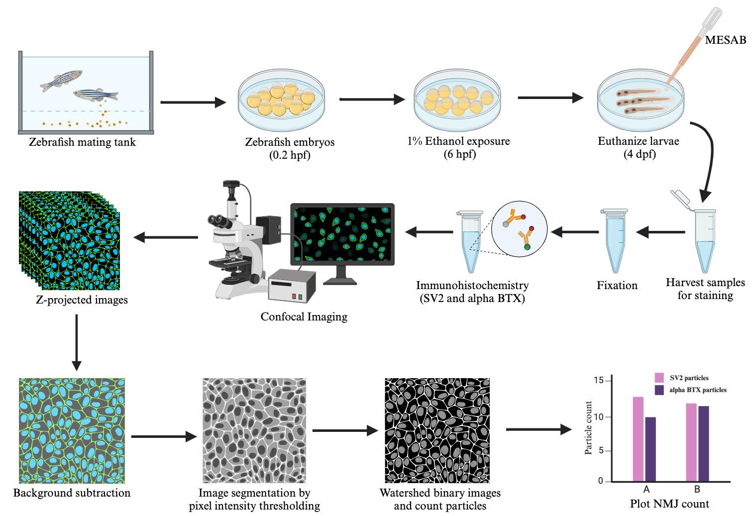
Keywords: Neuromuscular junctionsGraphical overview
Background
In vertebrates, the muscles of the face and neck are innervated by cranial motor neurons [1]. Communication between the brain and muscle is mediated through a specialized synapse known as the neuromuscular junction (NMJ). NMJs typically comprise three components: 1) the axonal end of the motor neuron, forming the presynaptic terminal; 2) the muscle endplate, forming the postsynaptic terminal; and 3) a synaptic cleft that lies between these two terminals. Neuromuscular communication occurs when acetylcholine, released from the presynaptic terminal into the synaptic cleft, binds acetylcholine receptors clustered in the postsynaptic terminal [2]. Alteration in NMJ morphology or distribution can lead to reduced synaptic transmission and result in neuromuscular disease. Zebrafish has emerged as an excellent model to study neuromuscular pathologies [3]. However, characterization and quantification of NMJs in the cranial muscles of zebrafish can be particularly challenging due to the anatomical complexity of the head.
Previous studies involving the quantification of NMJs in the cranial muscles were primarily carried out manually. Manual counting is arduous and can lead to individual bias and subjectivity. Some recent studies have carried out automated quantification using image analysis tools. However, most of these studies were carried out in somites of the zebrafish trunk region [4,5]. Unlike the head, the muscles of the trunk have a simpler, reiterated anatomy. Another study employed Imaris software for surface rendering with automatic thresholding to characterize the NMJs in the cranial musculature [6]. This method is useful for studying the number, shape, and architecture of NMJs. However, this also requires buying licensed software, making it inaccessible to some labs. Also, most of these studies use auto-thresholding, which can change the cutoff value for thresholding in individual images, unintentionally introducing errors [7].
Here, we developed a protocol for NMJ visualization and quantification in the cranial muscles using FIJI/ImageJ software, which is free of cost [8]. We immunolabel the presynaptic and postsynaptic terminals using SV2 antibody and alpha-bungarotoxin, respectively. We then capture high-resolution images of NMJs using confocal microscopy. Using the Area Selection tool, we crop out a region of specific dimensions containing the muscles of interest. We then use the Rolling Ball Background Subtraction plugin, Global Thresholding, and Watershed plugin to segment the images. Instead of auto-thresholding, we set the same cutoff value for thresholding each image, ensuring uniformity across all images. The number of particles in the segmented images is then counted using the Analyze Particles tool. We have used this protocol to investigate the effect of alcohol on NMJ count in a specific set of cranial muscles. However, the method can be applied to other cranial and trunk muscles of zebrafish. The method can also be used to quantify NMJs in other organisms like chickens and mice. Additionally, we used this method with 20× magnification for NMJ counting, but the method could readily be adapted for analyzing images of other magnifications. This method is broadly applicable to quantify other fluorescently labeled particles such as apoptotic cells, proliferating cells, or cells in general by counting DAPI-stained nuclei.
Materials and reagents
Biological materials
1. Zebrafish (Animal husbandry, Eberhart Lab, University of Texas at Austin, USA)
Reagents
1. Alpha-bungarotoxin (α-BTX) Alexa Fluor 647 conjugated (Invitrogen, catalog number: B35450)
2. Bovine serum albumin (BSA) (Sigma-Aldrich, catalog number: A4503, CAS: 9048-46-8)
3. Calcium chloride dihydrate (CaCl2·2H2O) (Sigma, catalog number: C8106, CAS: 10035-04-8)
4. Dimethyl sulfoxide (DMSO) (EMD Millipore Corp., catalog number: 317275, CAS: 67-68-5)
5. Ethanol (PHARMO, Ethyl Alcohol 100%, catalog number: 111000200, CAS: 64-17-5)
6. Goat anti-mouse IgG, Alexa Fluor 488 (secondary antibody) (Invitrogen, catalog number: A-11029)
7. Magnesium sulfate heptahydrate (MgSO4·7H2O) (Sigma-Aldrich, catalog number: 230391, CAS: 10034-99-8)
8. MESAB/Tricaine methanesulfonate (Syndel, SYNCAINE/MS 222, FDA approved)
9. Methanol (Fisher Chemical, catalog number: A412-4, CAS: 67-56-1)
10. Methylcellulose (Sigma-Aldrich, catalog number: M0387, CAS: 9004-67-5)
11. Normal goat serum (NGS) (Jackson ImmunoResearch Laboratories, catalog number: 005-000-121)
12. Paraformaldehyde (PFA) (Alfa Aesar, catalog number: A11313, CAS: 30525-89-4)
13. Phosphate-buffered saline (PBS) (Sigma-Aldrich, catalog number: P5368-10PAK)
14. Potassium chloride (KCl) (Fisher chemicals, catalog number: P217, CAS: 7447-40-7)
15. Potassium phosphate dibasic (K2HPO4) (Sigma-Aldrich, catalog number: P3786, CAS: 7758-11-4)
16. Sodium bicarbonate (NaHCO3) (Sigma-Aldrich, catalog number: S5761, CAS: 144-55-8)
17. Sodium chloride (NaCl) (CHEM-IMPEX INT’L INC., catalog number: 30070, CAS: 7647-14-5)
18. Sodium phosphate dibasic (Na2HPO4) (Acros organics, catalog number: 42437, CAS: 7558-79-4)
19. Synaptic vesicle 2A (SV2) antibody (Developmental Studies Hybridoma Bank, Antibody Registry ID: AB_2315387)
20. Triton X-100 (Triton X) (MP Biomedicals, catalog number: 194854, CAS: 9002-93-1)
Solutions
1. 10× PBS (See Recipes)
2. 1× PBT (See Recipes)
3. 4% PFA (See Recipes)
4. 25% methanol (See Recipes)
5. 50% methanol (See Recipes)
6. 75% methanol (See Recipes)
7. 20× embryo medium stock (See Recipes)
8. 500× sodium bicarbonate (See Recipes)
9. Embryo medium (See Recipes)
10. 1% ethanol (See Recipes)
11. Incubation buffer (See Recipes)
12. Blocking buffer (See Recipes)
13. Ethyl 3 Aminobenzoate methyl sulfonate salt (MESAB)/tricaine solution (See Recipes)
Recipes
1. 10× PBS
| Reagent | Final concentration | Quantity or Volume |
|---|---|---|
| Phosphate-buffered saline | 10× | 1 packet |
| ddH2O | n/a | Up to 100 mL |
| Total | n/a | 100 mL |
2. 1× PBT
| Reagent | Final concentration | Quantity or Volume |
|---|---|---|
| 10× PBS | 1× | 5 mL |
| Triton X | 0.5% (v/v) | 250 µL |
| ddH2O | n/a | Up to 50 mL |
| Total | n/a | 50 mL |
3. 4% PFA
*Note: Add PFA to 400 mL of ddH2O and heat and stir in a fume hood until the solution clears (do not heat at more than 60 °C). Add 50 mL of 10× PBS and adjust the pH to 7.4. Add ddH2O up to a total of 500 mL.
| Reagent | Final concentration | Quantity or Volume |
|---|---|---|
| 10× PBS | 1× | 50 mL |
| PFA | 4% (w/v) | 20 g |
| ddH2O | n/a | 450 mL* |
| Total | n/a | 500 mL |
Store 4% PFA at -20 °C.
4. 25% methanol
| Reagent | Final concentration | Quantity or Volume |
|---|---|---|
| Methanol | 25% (v/v) | 1 mL |
| 1× PBT | 75% (v/v) | 3 mL |
| Total | n/a | 4 mL |
5. 50% methanol
| Reagent | Final concentration | Quantity or Volume |
|---|---|---|
| Methanol | 50% (v/v) | 2 mL |
| 1× PBT | 50% (v/v) | 2 mL |
| Total | n/a | 4 mL |
6. 75% Methanol
| Reagent | Final concentration | Quantity or Volume |
|---|---|---|
| Methanol | 75% (v/v) | 3 mL |
| 1× PBT | 25% (v/v) | 1 mL |
| Total | n/a | 4 mL |
7. 20× embryo medium stock
| Reagent | Final concentration | Quantity or Volume |
|---|---|---|
| NaCl | 0.3 M | 17.5 g |
| KCl | 10.06 mM | 0.75 g |
| CaCl2·2H2O | 19.72 mM | 2.9 g |
| K2HPO4 | 2.35 mM | 0.41 g |
| Na2HPO4 | 1 mM | 0.142 g |
| MgSO4·7H2O | 19.88 mM | 4.9 g |
| ddH2O | n/a | Up to 1 L |
| Total | n/a | 1 L |
Filter-sterilize the solution.
8. 500× sodium bicarbonate
| Reagent | Final concentration | Quantity or Volume |
|---|---|---|
| NaHCO3 | 0.35 M | 0.3 g |
| ddH2O | n/a | 10 mL |
9. Embryo medium
| Reagent | Final concentration | Quantity or Volume |
|---|---|---|
| 20× embryo medium stock | 1× | 50 mL |
| 500× sodium bicarbonate | 1× | 2 mL |
| ddH2O | n/a | 948 mL |
| Total | n/a | 1 L |
10. 1% Ethanol
| Reagent | Final concentration | Quantity or Volume |
|---|---|---|
| Ethanol | 1% (v/v) | 400 µL |
| Embryo medium | 99% (v/v) | 39.6 mL |
| Total | n/a | 40 mL |
11. Incubation buffer
| Reagent | Final concentration | Quantity or Volume |
|---|---|---|
| 10× PBS | 1× | 5 mL |
| BSA | 1% (w/v) | 500 mg |
| DMSO | 1% (v/v) | 500 µL |
| Triton X-100 | 0.5% (v/v) | 250 µL |
| ddH2O | n/a | Up to 50 mL |
| Total | n/a | 50 mL |
12. Blocking buffer
| Reagent | Final concentration | Quantity or Volume |
|---|---|---|
| Incubation buffer | 96% (v/v) | 960 µL |
| Normal goat serum | 4% (v/v) | 40 µL |
| Total | n/a | 1,000 µL |
13. MESAB/tricaine solution
| Reagent | Final concentration | Quantity or Volume |
|---|---|---|
| Na2HPO4 | 0.8 % (w/v) | 4 g |
| MESAB salt | 0.4 % (w/v) | 2 g |
| ddH2O | n/a | Up to 500 mL |
| Total | n/a | 500 mL |
Adjust pH between 7.0 and 7.2.
Laboratory supplies
1. Petri dishes 100 mm × 20 mm (Falcon, catalog number: 353003)
2. Micropipettes (Sigma-Aldrich, catalog number: FA10006M-1EA)
3. Pipette pumps (Fisher Scientific, catalog number: 13-683C)
4. 1.7 mL microcentrifuge tubes (Fisher Scientific, catalog number: 07-200-535)
Equipment
1. Confocal microscope (Zeiss, model: LSM 980)
2. Stereoscope (Leica, model: KL 300 LED)
Software and datasets
1. ImageJ2 v2.14.0/1.54f (available free of cost from https://fiji.sc/, 07/07/2023)
2. Prism v9.5.0 (GraphPad, 12/06/2022)
Procedure
Here, we describe a stepwise protocol to visualize and quantify the NMJs in the cranial muscles of zebrafish larvae at 4 days post fertilization. This protocol has been used to compare the number of NMJs in ethanol-exposed and unexposed zebrafish [9]. The protocol can be adapted for comparing NMJs at other times, in other conditions, and in other muscle(s).
A. Sample preparation
1. Alcohol treatment of zebrafish embryos
a. Harvest wildtype zebrafish embryos and incubate at 28 °C in 40 mL of embryo medium (see Recipes) in a 100-mm Petri dish with a maximum number of 100 embryos per dish. Allow the embryos to develop until shield stage, which is at about 6 h post fertilization (6 hpf). Zebrafish staging has been previously described [10].
b. At 6 h post-fertilization, freshly prepare 40 mL of 1% ethanol in embryo medium (see Recipes). Replace the embryo medium in the experimental dish with the freshly prepared 1% ethanol solution. Leave the control dish with embryo medium untreated. Place the experimental and control dishes in the incubator at 28 °C and allow the embryos to develop until 4 days post fertilization (4 dpf). Keep the dishes with the developing zebrafish embryos clean by periodically (daily at a minimum) removing any dead embryos or chorions shed during hatching.
2. Fixation
a. At 4 dpf, harvest 15 fish each from the control and experimental dishes. To harvest zebrafish, euthanize using MESAB/tricaine (see Recipes) in embryo medium. Using a graduated dropper, add MESAB/tricaine to a final concentration of 200–300 mg/L. Transfer the euthanized zebrafish from the control and experimental dishes to 1.7 mL microcentrifuge tubes using a pipette pump.
b. Remove any excess liquid from the microcentrifuge tubes using a pipette pump.
c. Add 1 mL of 4% PFA solution (see Recipes) and place the microcentrifuge tubes on a nutator at 4 °C for overnight fixation.
Caution: PFA is toxic and should be disposed of according to institutional regulations. Proper care must be taken while working with PFA (e.g., use of gloves and working in a chemical hood).
d. After overnight fixation, remove the 4% PFA solution from the tubes and wash the zebrafish larvae with 1 mL of 1× PBS for 5 min on the nutator at room temperature (wash at least twice to ensure complete removal of PFA).
Note: After the wash step, the zebrafish are ready for the immunohistochemical staining. However, to store the zebrafish larvae until later use, carry out methanol dehydration as described in the next step.
3. Methanol dehydration for long-term storage (optional)
a. For methanol dehydration, prepare 25%, 50%, and 75% methanol solutions in 1× PBT (see Recipes). Dehydrate larvae with serially diluted methanol solutions (1× PBT, 25%, 50%, 75%, and then 100% methanol) by washing the larvae in 1 mL of each solution for 5 min on the nutator at room temperature. Replace 100% methanol with 1 mL of cold 100% methanol. Store the zebrafish larvae at -20 °C.
Pause point: The dehydrated larvae can be stored in 70% methanol solution at 4 °C for a week or in 100% methanol at -20 °C for a maximum of 6 months.
b. Rehydrate the zebrafish larvae stored in methanol at -20 °C. Wash once for 5 min with the serially diluted methanol solutions (75%, 50%, 25%, and then 1× PBT) on the nutator at room temperature.
B. Immunohistochemistry for NMJs in cranial muscles
1. Freshly prepare incubation buffer (see Recipes) and wash four times in 1 mL of incubation buffer for 20 min each on the nutator at room temperature.
2. Freshly prepare blocking buffer (see Recipes). Wash the zebrafish once with 500 µL of blocking buffer for 30 min on the nutator at room temperature.
3. Prepare 250 µL of primary antibody solution in blocking buffer. For labeling the presynaptic terminals, use primary antibody against synaptic vesicle 2A (see Reagents) to get a final concentration of 5 µg/mL. Replace the blocking buffer with primary antibody solution and place the microcentrifuge tubes on a nutator with gentle rocking at 4 °C for overnight incubation.
4. The following day, remove the primary antibody solution and wash the zebrafish larvae four times with 1 mL of incubation buffer for 20 min each on the nutator at room temperature.
5. Wash once with 500 µL of blocking buffer for 30 min on the nutator at room temperature.
6. Prepare 250 µL of anti-mouse IgG Alexa Fluor 488 secondary antibody solution in blocking buffer at 1:500 dilution by adding 0.5 µL of secondary antibody to 250 µL of blocking buffer. Also, add 1 µL of alpha-bungarotoxin (α-BTX) Alexa Fluor 647 conjugated primary antibody to obtain a 1:250 dilution (see Reagents for details on antibodies).
7. Replace the blocking buffer with the antibody solution and cover the tubes with aluminum foil to protect from the light. Place the tubes on an incubator at 4 °C for overnight incubation with gentle rocking.
8. The following day, remove the antibody solution from the tubes and wash three times with 1 mL of 1× PBT for 5 min each on the nutator at room temperature.
9. Fix the immunostained zebrafish larvae for 20 min by washing in 4% PFA on the nutator at room temperature.
10. Wash twice in 1 mL of 1× PBT for 5 min each on the nutator at room temperature.
11. Replace the 1× PBT solution with 1 mL of 1× PBS solution. The zebrafish larvae are ready to be imaged.
Pause point: Immunostained larvae in 1× PBS can be stored at 4 °C covered in foil (protected from light) for a week before imaging.
Note: It is recommended that they are imaged as soon as possible after immunostaining to prevent loss of fluorescence.
C. Confocal imaging
Mount the immunolabeled zebrafish to collect ventral images in 0.2% agarose and 3% methylcellulose as previously described [11]. To mount the samples, add a drop of methylcellulose using a wooden applicator in the middle of a triple-bridged coverslip. Using a pipette pump, transfer the immunolabeled zebrafish from 1× PBS to 0.2% agarose. Next, transfer the zebrafish along with some agarose solution to the methylcellulose drop. For an upright microscope, orient the zebrafish in a ventral-upward position using a capillary poker and carefully place the coverslip on the top. Acquire bidirectional confocal Z-stacks at 20× magnification. We used the Zeiss LSM 980 microscope with 20× objective lens, 1,024 × 1,024 frame size, and 4× averaging. Confocal stacks were Z-projected with maximum intensity as shown in Figure 1 for further image analyses described in section D.
Note 1: Make sure to image through the entire depth of the brachial region to capture all muscle fibers. Most ventral cranial muscles, such as the intermandibularis posterior and interhyoideus and hyohyoideus inferior muscles, are fairly superficial. However, the intermandibularis anterior, hyohyoideus superior, sternohyoideus, and adductor mandibularis muscles are much deeper. Make sure to image through their depth to capture the entire muscle. For 4 dpf zebrafish, a depth of 60 µm should be sufficient to capture all ventral branchial muscles shown in Figure 1A.
Note 2: Make sure that all images for analysis are captured using the same confocal settings such as laser intensity, gain, frame size, averaging, etc.
Note 3: Also, the distance between two consecutive Z-slices should be the same across all images for comparison and should not be more than 2 µm for looking at the NMJs.
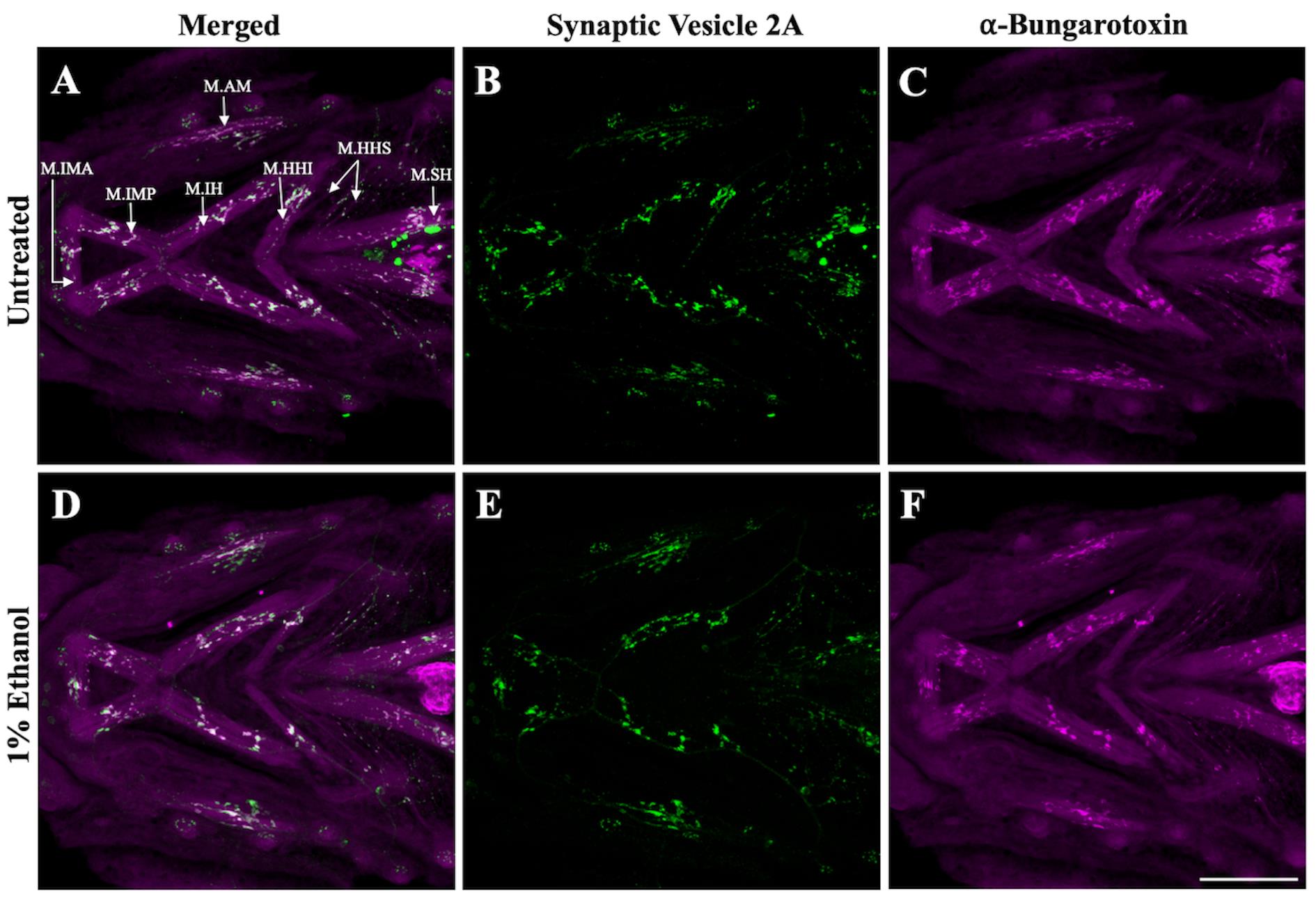
Figure 1. Confocal images of ventral cranial muscles immunostained with synaptic vesicle 2A (SV2) and alpha-bungarotoxin (α-BTX) in zebrafish at 4 dpf. A, D. Merged channels with SV2-stained presynaptic terminals (in green) and α-BTX-stained postsynaptic terminals (in magenta) in untreated and ethanol-treated zebrafish. Ventral cranial muscles in zebrafish larvae at 4 dpf, as previously described [12], are shown in A: M.IMA: intermandibularis anterior muscle; M.IMP: intermandibularis posterior muscle; M.IH: interhyoideus muscle; M.AM: adductor mandibulae muscle; M.HHI: hyohyoideus inferior muscle; M.HHS: hyohyoideus superior muscle; M.SH: sternohyoideus muscle. B, E. SV2-labeled presynaptic terminals in untreated and alcohol-exposed zebrafish. C, F. α-BTX-labeled postsynaptic terminals in untreated and alcohol-exposed zebrafish. Scale bar = 100 µm.
D. Image analysis using FIJI/ImageJ software
To study the size and distribution of presynaptic and postsynaptic terminals in the ventral cranial muscles of zebrafish larvae, FIJI/ImageJ software can be used. Analyses can be carried out for one or more cranial muscles of interest. In this example, the quantification of the NMJs in four cranial muscles, the intermandibularis anterior, intermandibularis posterior, interhyoideus, and hyohyoideus inferior muscles has been carried out.
1. Area selection to pick the muscles of interest:
a. Open the image file with ImageJ software. To Z-project the image, select the image and choose Image → Stacks → Z project from the ImageJ menu options. Select Max Intensity as the Projection type and click OK on the ZProjection dialog box.
b. To pick the muscles of interest, use the rectangular selection tool to crop out a region of 300 × 180 µm^2 (= 750 × 450 in pixel units) containing intermandibularis anterior, intermandibularis posterior, interhyoideus, and hyohyoideus inferior muscles. To specify the dimensions for the area of interest, choose Edit → Selection → Specify. The Specify dialog box will appear. Check the Scaled unit (microns) box and enter 300 and 180 as the Width and Height, respectively, as illustrated in Figure 2A. Other sizes can be used depending on the researcher’s specific interests. Click OK to proceed.
c. Using the arrow tool, drag the rectangle of the specified dimensions to the desired location to select the muscles of interest. For instance, here, the rectangle outlines the intermandibularis anterior, intermandibularis posterior, interhyoideus, and hyohyoideus inferior muscles (Figure 2A).
d. To crop out the selected region, choose Image → Crop or Image → Duplicate. Only the selected region will be included in the duplicated image (Figure 2B). All further steps will be carried out on this duplicated or cropped image with the muscles of our interest.
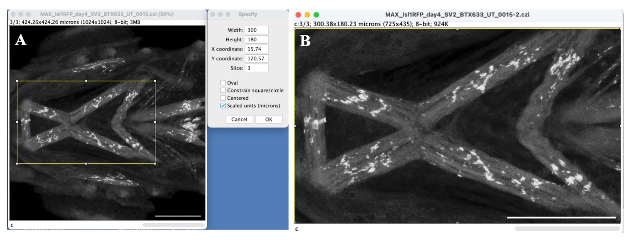
Figure 2. Area selection to select a region of specific dimensions. A. Z-projected image with the rectangular selection (in yellow) of 300 µm in width and 180 µm in height. The dialog box on the right shows the values specified for width and height in scaled units (microns). B. Cropped region of the image with 300 × 180 µm^2 selected area for analysis. Scale bar = 100 µm.
2. Background subtraction: To correct the uneven background illumination, use the Rolling ball background subtraction plugin.
a. To apply the method, select Process → Subtract Background from the ImageJ menu options. The Subtract Background dialog box will appear. Enter the Rolling ball radius and press OK.
b. To determine the Rolling ball radius, measure the length of the largest object (i.e., NMJ) by using the Line selection tool on ImageJ. Draw a line connecting two dots that defines the length of the largest object on the image and select Analyze → Measure to get the length in microns for a scaled image (Figure 3). Here, the largest length was found to be ~10 (9.199) µm.
c. For this image, pixel size = 0.4 µm in length and breadth. Thus, 10 µm = 25 pixels. Enter 25 as the Rolling ball radius in pixels and click OK. A Process Stack? dialog box will appear. To apply the background subtraction to both SV2 and α-BTX channels, select Yes to Process all images? on the Process Stack? dialog box. Figure 4 shows the images before and after correcting their background illumination using the Rolling ball background subtraction plugin.
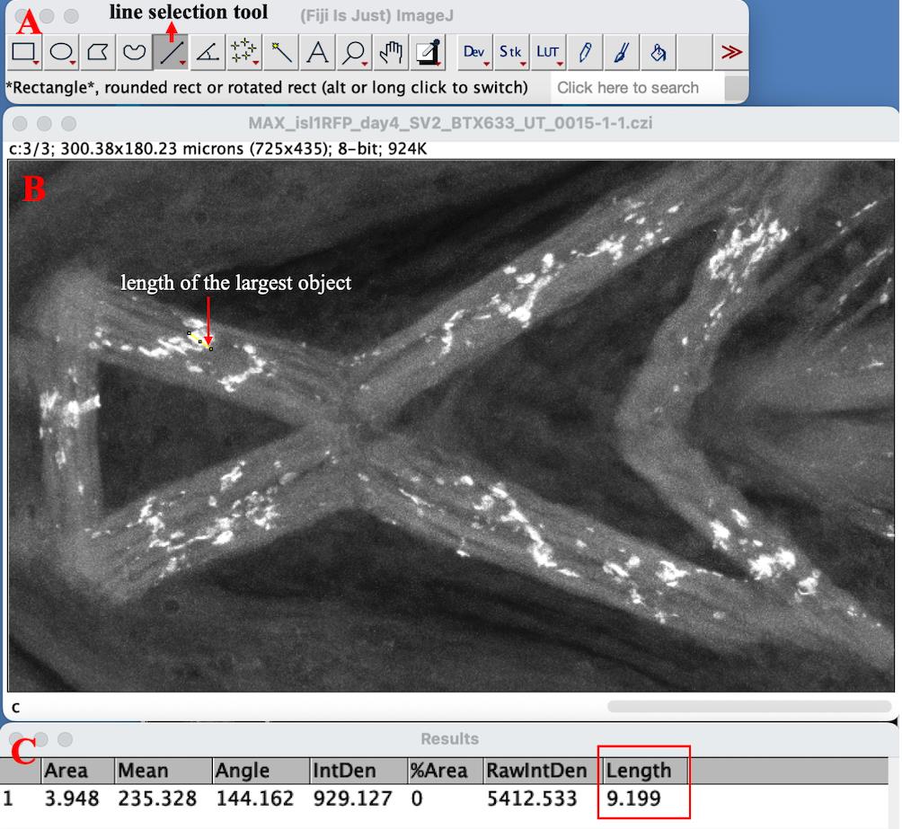
Figure 3. Determining the rolling ball radius by measuring the length of the largest object on the image. A. The red arrow shows the line selection tool. B. Line drawn with the line selection tool to denote the length of the largest object on the image. C. Result table displaying the length of the line drawn as 9.199 µm (highlighted by the red rectangle).
Note 1: To find the pixel size of your image, select the image and choose Image → Properties from the ImageJ menu options.
Note 2: In theory, the rolling ball radius is determined by measuring the length of the largest object or particle in the image that is considered a true signal and not part of the background. However, in practice, the optimum radius can be worked out by trying different values using the Preview option on the Subtract Background window. If the value is too large, it might not fix the uneven background; on the other hand, a very small radius can take away parts of the real signal (synaptic terminals in this case).
Note 3: The rolling ball radius can be different for different channels. So, determine the radius for both channels separately using step D2b. However, here, we found that the largest particles on both channels were approximately the same length. Thus, we processed both channels using the same radius.
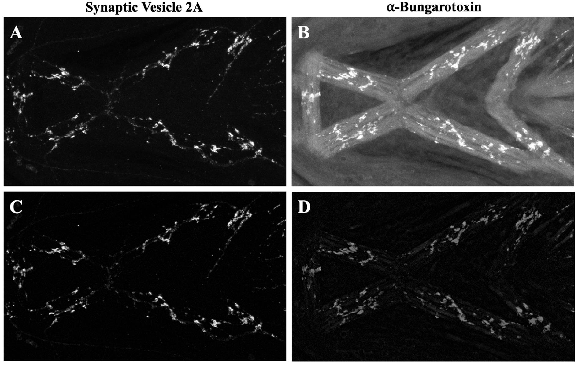
Figure 4. Background subtraction on SV2 and α-BTX channels. A, B. Images of SV2- and α-BTX-labeled objects before background subtraction. C, D. Images of SV2- and α-BTX-labeled objects after correcting the uneven background illumination using the rolling ball background subtraction method.
3. Image segmentation:
The aim of this step is to separate the objects or particles (foreground) from the background by global thresholding using pixel intensity.
a. Begin by splitting the SV2 and α-BTX channels from the image. To split channels, choose Image → Color → Split channels.
Note: You can threshold without splitting the channels. However, it is recommended to split the channels into different image windows.
b. Then, choose Image → Adjust → Threshold. A Threshold dialog box will appear. Select the α-BTX channel and click on the Set option on the Threshold dialog box to enter a cutoff value for thresholding (indicated by the red arrow in Figure 5).
c. Enter the Lower threshold level as 45 (as indicated by the black arrow in Figure 5) on the Set Threshold Levels dialog box and click OK. This step will divide the image into two classes of pixels: pixels greater than the cutoff value (foreground in red) and pixels less than the cutoff value (background in black).
Note: You can invert colors for foreground and background on the Threshold dialog box.
d. Click Apply on the Threshold dialog box to convert the image to a binary image.
e. Repeat steps D3b–d on the SV2 channel to similarly create a binary image for the SV2 channel.
Note: The thresholding can be carried out using manual or auto-thresholding options. An auto threshold is often considered more reproducible and unbiased. However, thresholding works on the basis of distributing pixel intensities on the images. If the distribution changes, thresholding will change too. Thus, even auto threshold can introduce errors by changing the thresholding cutoff levels. In practice, one should determine the method and cutoff value for thresholding using positive and negative controls. Count the number of objects in one or more control images (in a blinded manner) and then apply different thresholding methods to compare the object count with the control images. Determine the method that works best for your experiments.
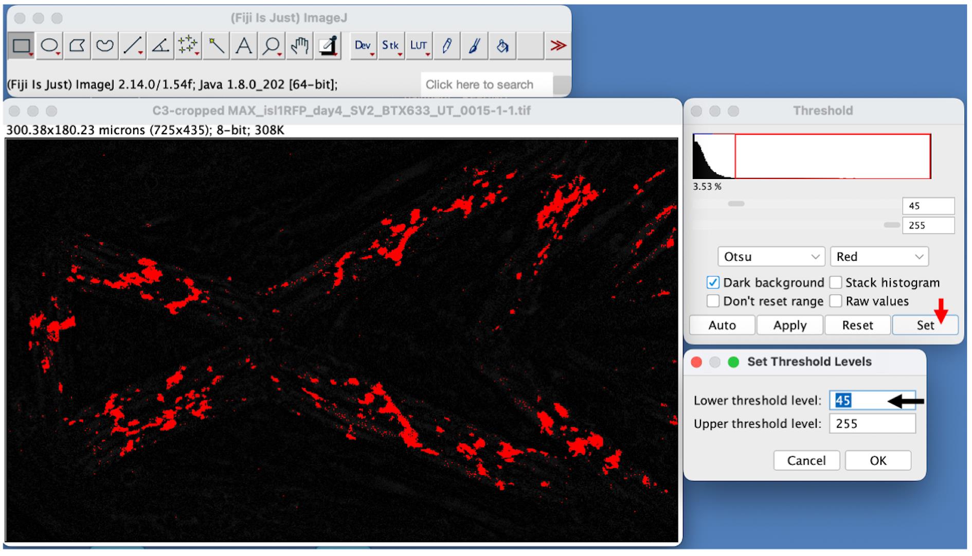
Figure 5. Image segmentation by using pixel intensity thresholding. Here, the objects are represented in red on a black background. The red arrow on the Threshold dialog box on the right shows the Set option. Clicking the Set option opens the Set Threshold Levels dialog box. The black arrow on the Set Threshold Levels dialog box shows the value for the lower threshold level.
4. Apply the watershed plugin on the binary images to separate out any overlapping particles. Select the binary image for α-BTX channel and choose Process → Binary → Watershed from the ImageJ menu. Repeat this step for the binary image generated for the SV2 channel. As illustrated in Figure 6, the algorithm will separate out the connected objects (compare the regions pointed out by the arrows in panels C and F).
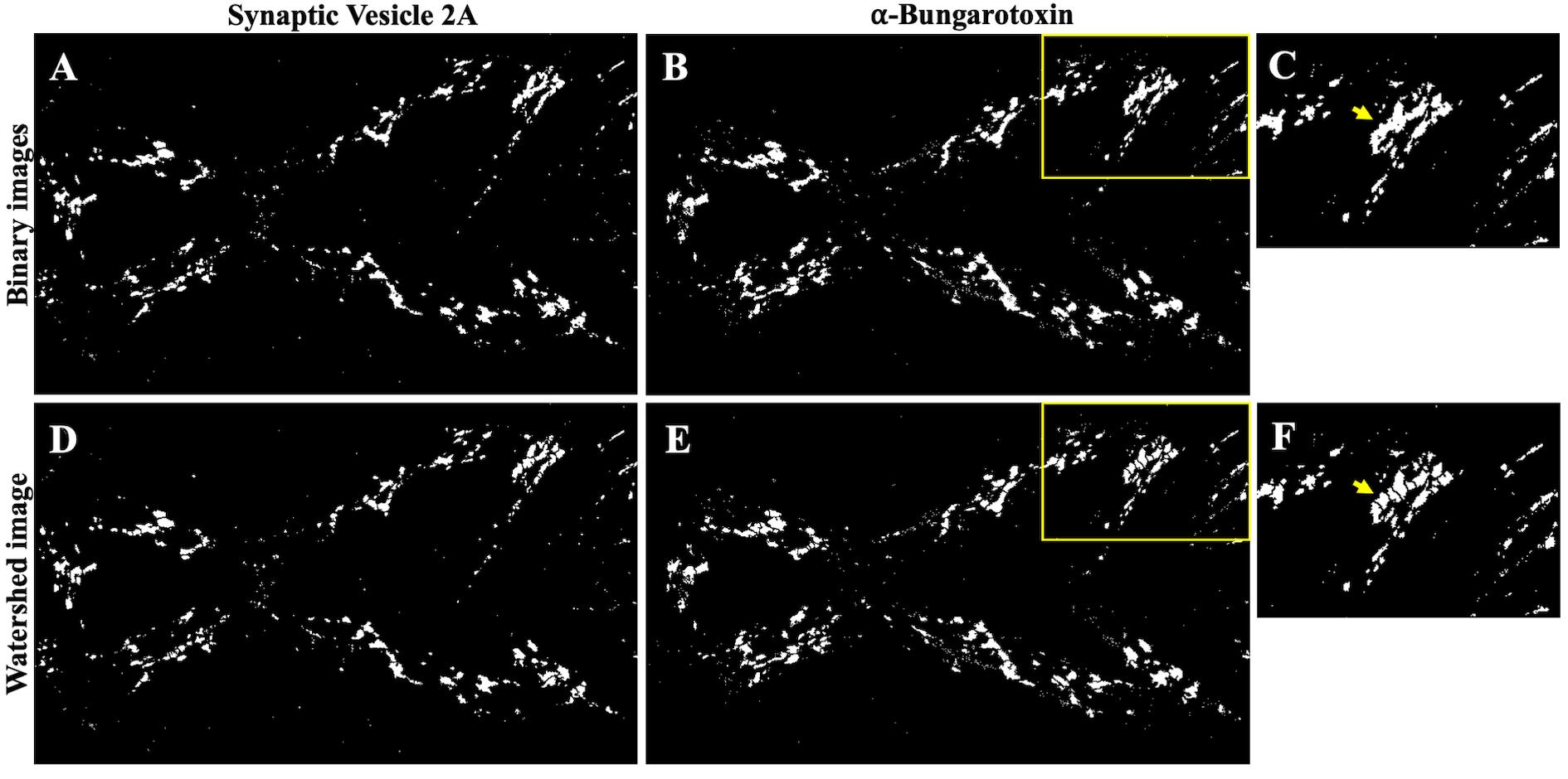
Figure 6. Watershed method for separating two or more connected objects. A, B. Binary images of SV2 and α-BTX channels generated after the image thresholding in step D3. D, E. Watershed images of A and B after applying the watershed plugin. C, F. Insets from B and E. The arrow in F indicates the objects separated by the watershed method.
5. Counting particles:
In this step, use the Analyze Particles tool to count the number of objects or particles in the segmented images of α-BTX and SV2 channels.
a. Click on the segmented image generated after step D4 and choose Analyze → Analyze Particles. The Analyze Particles dialog box appears. This tool allows us to filter out particles of specific size and circularity range.
b. To count the number of SV2- and α-BTX-labeled particles with an area greater than 8 µm2, input 8-Infinity for Size (micron^2) on the Analyze Particles dialog box as illustrated in Figure 7. We determined the 8 µm2 value after trying out multiple values. At this cutoff, we were able to eliminate most particles that were visibly outside the muscles and thus were not NMJs.
c. NMJs are not necessarily circular, so leave the Circularity as 0.00–1.00 (value 0 denotes a line, and value 1 indicates a perfect round object). Thus, this option will allow us to select particles of all shapes.
d. Choose Masks from the Show dropdown menu and check the boxes Summarize and Overlay on the Analyze particles dialog box. Click OK to find the object count on a result table.
e. Record the particle count for SV2- and α-BTX-labeled objects for all untreated and ethanol-exposed zebrafish samples. Figure 8 shows representative images after the area selection, segmentation, and analyze particles methods.
Note 1: A macro can be recorded on ImageJ using the Macro recorder to automate these set of commands. Alternatively, repeat these steps manually for both SV2 and α-BTX channels on untreated and ethanol-exposed zebrafish images, keeping all parameters of image analyses and image acquisition the same across all images.
Note 2. This method has been used here to separately analyze presynaptic and postsynaptic particles. However, the protocol can be modified to count the number of NMJs by looking at the co-localized SV2 and α-BTX particles using the AND function on Image Calculator. After correcting the background illumination in step D2 of this protocol, split the SV2 and α-BTX channels from the image. To split channels, choose Image → Color → Split Channels. Then, go to Image Calculator by selecting Process → Image Calculator. An Image Calculator dialog box will appear. Choose SV2 channel as Image1 and α-BTX channel as Image2. Select AND as the operation, check on the Create new window box, and click OK. A new image will be generated with only co-localized SV2 and α-BTX particles. Segment this image and analyze particles (using steps D3, 4, and 5) to get the NMJ count.
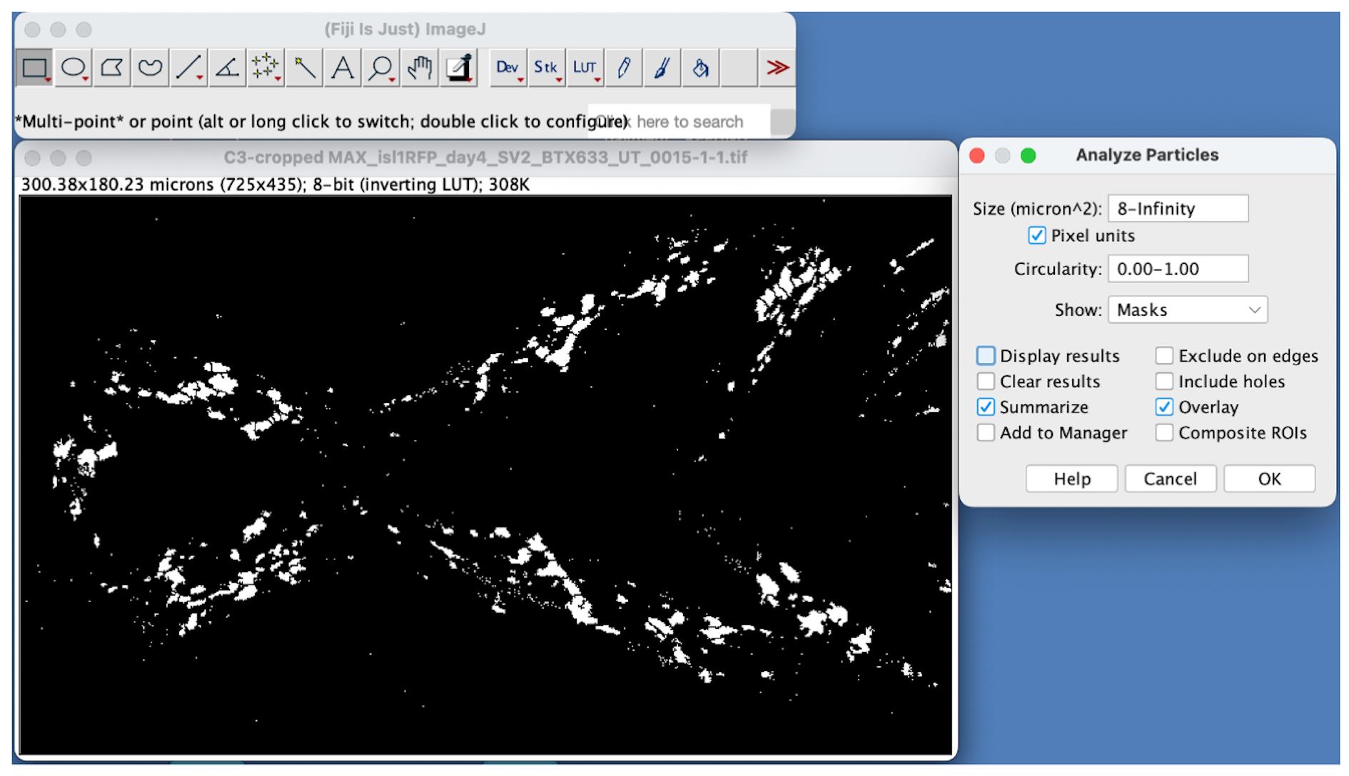
Figure 7. Counting particles using the Analyze Particles tool on ImageJ. Define the size and circularity range on the Analyze Particles dialog box. Here, particles greater than 8 µm2 were filtered out using this tool.
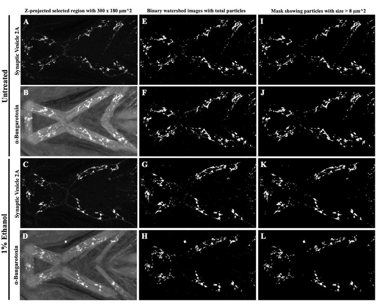
Figure 8. Representative images generated after applying the area selection, segmentation, and particle count methods for SV2- and α-BTX-labeled objects in untreated and alcohol-treated zebrafish. A–D. Cropped region of interest with an area of 300 × 180 µm2 after applying the area selection tool to untreated (A, B) and ethanol-treated (C, D) images. E–H. Segmented images with objects in white on a black background. Binary images of untreated (E, F) and ethanol-treated (G, H) SV2 and α-BTX channels obtained after manual thresholding using a specific cutoff value of 45 as the lower threshold level. I–L. Selected objects with size greater than 8 µm2 included in the final count using the Analyze Particles tool in untreated (I, J) and ethanol-treated (K, L) SV2 and α-BTX images.
Data analysis
Plot the number of recorded particles, presynaptic terminals (SV2-labeled particles), and postsynaptic terminals (α-BTX-labeled particles) in the control and alcohol-exposed zebrafish samples using GraphPad Prism software. Enter the data in a Grouped table format and run a two-way ANOVA with Tukey’s multiple comparisons correction to compare the number of presynaptic and postsynaptic terminals in the untreated and ethanol-exposed zebrafish. Present the data as mean ± SEM. We have previously used this method with n = 14 for each treatment. The detailed description can be found in section 4.10 and Figure 11S of Ghosal et al., 2023. Using this protocol, we found a reduction in the number of postsynaptic terminals relative to presynaptic terminals in alcohol-treated zebrafish.
Validation of protocol
This protocol or parts of it has been used and validated in the following research article:
Ghosal et al. [9]. Embryonic ethanol exposure disrupts craniofacial neuromuscular integration in zebrafish larvae. Front Physiol (Figure 11, panels G–S).
Acknowledgments
This work was funded by NIH/NIAAA R01AA023426, NIH/NIDCR R35DE029086, and NIH/NIAAA R01AA031346 to JKE. This protocol was originally described and validated by Ghosal et al. [9].
Competing interests
The authors declare no competing interests. This work was conducted in the absence of any commercial or financial relationships.
Ethical considerations
The zebrafish lines used for this study were housed and raised in the University of Texas at Austin based on previously described protocols [13]. All protocols were approved by the Institutional Animal Care and Use Committee.
References
- Guthrie, S. (2007). Patterning and axon guidance of cranial motor neurons. Nat Rev Neurosci. 8(11): 859–871. https://doi.org/10.1038/nrn2254
- Jing, L., Gordon, L. R., Shtibin, E. and Granato, M. (2010). Temporal and Spatial Requirements of unplugged/MuSK Function during Zebrafish Neuromuscular Development. PLoS One. 5(1): e8843. https://doi.org/10.1371/journal.pone.0008843
- Singh, J. and Patten, S. A. (2022). Modeling neuromuscular diseases in zebrafish. Front Mol Neurosci. 15: e1054573. https://doi.org/10.3389/fnmol.2022.1054573
- Singh, J., Pan, Y. E. and Patten, S. A. (2023). NMJ Analyser: a novel method to quantify neuromuscular junction morphology in zebrafish. Bioinformatics. 39(12): e1093. https://doi.org/10.1093/bioinformatics/btad720
- Lescouzères, L., Bordignon, B. and Bomont, P. (2022). Development of a high-throughput tailored imaging method in zebrafish to understand and treat neuromuscular diseases. Front Mol Neurosci. 15: e956582. https://doi.org/10.3389/fnmol.2022.956582
- Luderman, L. N., Michaels, M. T., Levic, D. S. and Knapik, E. W. (2022). Zebrafish Erc1b mediates motor innervation and organization of craniofacial muscles in control of jaw movement. Dev Dyn. 252(1): 104–123. https://doi.org/10.1002/dvdy.511
- Nijhof, B., Castells-Nobau, A., Wolf, L., Scheffer-de Gooyert, J. M., Monedero, I., Torroja, L., Coromina, L., van der Laak, J. A. and Schenck, A. (2016). A New Fiji-Based Algorithm That Systematically Quantifies Nine Synaptic Parameters Provides Insights into Drosophila NMJ Morphometry. PLoS Comput Biol. 12(3): e1004823. https://doi.org/10.1371/journal.pcbi.1004823
- Schindelin, J., Arganda-Carreras, I., Frise, E., Kaynig, V., Longair, M., Pietzsch, T., Preibisch, S., Rueden, C., Saalfeld, S., Schmid, B. et al. (2012). Fiji: an open-source platform for biological-image analysis. Nat Methods. 9(7): 676–82. https://doi.org/10.1038/nmeth.2019
- Ghosal, R., Borrego-Soto, G. and Eberhart, J. K. (2023). Embryonic ethanol exposure disrupts craniofacial neuromuscular integration in zebrafish larvae. Front Physiol. 14: e1131075. https://doi.org/10.3389/fphys.2023.1131075
- Kimmel C. B., Ballard W. W., Kimmel S. R., Ullmann B., Schilling T. F. (1995). Stages of embryonic development of the zebrafish. Dev Dyn. 203: 253–310. https://doi.org/10.1002/aja.1002030302
- McGurk, P. D., Lovely, C. B. and Eberhart, J. K. (2014). Analyzing Craniofacial Morphogenesis in Zebrafish Using 4D Confocal Microscopy. J Visualized Exp. 83: e51190. https://doi.org/10.3791/51190-v
- Schilling, T. F. and Kimmel, C. B. (1997). Musculoskeletal patterning in the pharyngeal segments of the zebrafish embryo. Development. 124(15): 2945–2960. https://doi.org/10.1242/dev.124.15.2945
- Westerfield M. (2000). The zebrafish book. A guide for the laboratory use of zebrafish (Danio rerio). 4th Edition. Eugene: University of Oregon Press.
Article Information
Publication history
Received: Oct 15, 2024
Accepted: Jan 2, 2025
Available online: Jan 26, 2025
Published: Feb 20, 2025
Copyright
© 2025 The Author(s); This is an open access article under the CC BY-NC license (https://creativecommons.org/licenses/by-nc/4.0/).
How to cite
Ghosal, R. and Eberhart, J. K. (2025). Quantification of Neuromuscular Junctions in Zebrafish Cranial Muscles. Bio-protocol 15(4): e5219. DOI: 10.21769/BioProtoc.5219.
Category
Developmental Biology > Morphogenesis > Cell structure
Cell Biology > Cell imaging > Confocal microscopy
Do you have any questions about this protocol?
Post your question to gather feedback from the community. We will also invite the authors of this article to respond.