Materials and reagents

96-well black/clear-bottom plate (Thermo Fisher Scientific, Nunc^TM, catalog number: 165305)
Collagen I, rat tail (Thermo Fisher Scientific, Gibco^TM, catalog number: A1048301)
Hoechst 33342 (Thermo Fisher Scientific, Invitrogen^TM, catalog number: H3570)
HEPES (Thermo Fisher Scientific, Gibco^TM, catalog number: 15630106)
Bovine serum albumin (BSA) (BioShop, catalog number: ALB001)
Recombinant human EGF (PeproTech, catalog number: AF-100-15)
Human FGF-acidic recombinant protein (Thermo Fisher Scientific, Gibco^TM, catalog number: PHG0014)
Heparin sodium salt from porcine intestinal mucosa (Merck, Sigma-Aldrich, catalog number: H3393)
Trametinib (LC laboratories, catalog number: T-8123)
PBS, pH 7.4 (Thermo Fisher Scientific, Gibco^TM, catalog number: 10010023)
Cell migration supplements (see Recipes)

Cell lines

SAS cell line was used as indicated. Cells were grown in Dulbecco’s modified Eagle medium (DMEM) with 10% fetal bovine serum (FBS), and 1% penicillin and streptomycin.

Recipes

Cell migration supplements
20 mM HEPES
0.1% BSA
5 ng/mL EGF or 25 ng/mL FGF1
10 U heparin

Equipment

Fluorescence microscope (Nikon Eclipse Ti)
96-well scratcher (can be replaced by 200 μL tip or toothpick)

Software

MATLAB (MathWorks, https://www.mathworks.com/products/matlab.html) with the image processing toolbox (access date, 8/1/2017)
Nikon NIS-Elements Viewer (Nikon image acquisition software) (access date, 9/21/2017)
Fiji from ImageJ (open resource software for image analysis) (access date, 8/1/2017)
Excel (Microsoft) (access date, 8/1/2017)

Procedure

Plate coating and cell seeding

Add 100 μL of collagen I (30 μg/mL, diluted in PBS) to the 96-well black/clear-bottom plate and put the plate in a 37 °C, 95% humidity incubator for 30–40 min.
Rinse the plate with 100 μL of PBS and aspirate the liquid in the plate thoroughly before use.
After that, plate SAS cells onto the plate. (The cell number should be controlled to 90%–100% confluency on the day performing cell migration.)
(Optional) Cells were infected with lentiviruses for 24 h and selected with antibiotics for 24–48 h.

Nucleus staining

Stain the cells with 1 μg/mL of Hoechst 33342 at 37 °C for 1 h for SAS cells.

Scratching (for wound-healing assay only)

Change the medium to 100 μL of pre-warmed PBS.
Scratch the cells with a scratcher (move the scratcher back and forth twice). This method is for a full 96-well plate and can be replaced by using toothpicks or 200 μL tips if only part of the 96 well plate is used.
After wound-scratching, wash the cells with 100 μL of PBS twice to remove cell fragments.

Drug treatment

Change the medium to serum-free DMEM medium (for SAS cells) containing cell migration supplements and drugs (we used trametinib 100 nM or DMSO).

Imaging

Place the cells in an acrylic incubator at 32 °C for SAS cells. The acrylic incubator is a chamber with CO₂ circulation [the temperature is lower than normal incubation (37 °C) to optimize the migration speed for analysis].
Use Nikon Eclipse Ti microscope for live-cell imaging. Take images every 10 min for a duration of 6–10 h. Our script is designed for pictures taken by 4× objective.

Data analysis

We process the image data through our MATLAB scripts. The schematic summary of how these images are processed is in Figure 1.

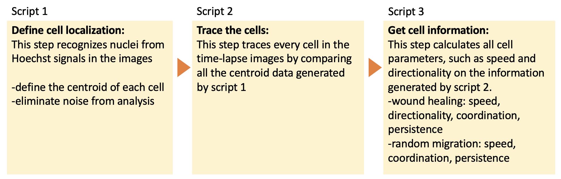
Figure 1. Schematic summary of data processing using MATLAB scripts

Description of MATLAB scripts and analysis

Define nuclei location: Z1_calcnuclei_adjustedPlateShift
This script defines the cell location in each image.
1. Open MATLAB, import data, and prepare the script.
2. Export images to working directory: an individual image is required for DAPI channel and time-lapse.
  Note: The file name should begin with “well + row number + column number” to fit our script. If not, this could be changed in line 13. All images should be exported as tiff files (Figure 2).
  
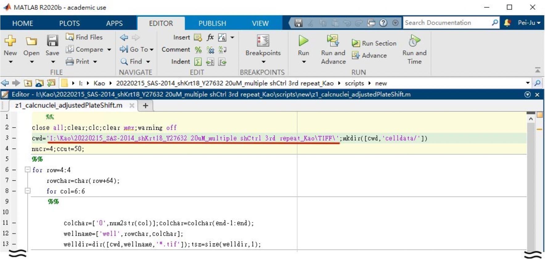
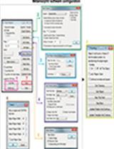
  Figure 2. Screenshot of Z1_calcnuclei_adjustedPlateShift user interface. Underlined is the path of exported tiff files. Note that the image file name in the folder should follow the rule: well + row number + column number + other details, e.g., WellA01_ChannelDAPI _Seq0000_ Z01_C1.tif (L12).
3. Open Z1_calcnuclei_adjustedPlateShift.m.
4. (Optional) Change the nuclear size in line 4. The nucleus size should be changed based on your cell line (in this case, we use 4 for SAS to best discriminate each cell).
5. Change the file path in line 3 and fill the row and column number based on your experimental setting in line 6 and 8. (In this case, we choose row B–G, and column 1–12, so we fill 2:7 for row and 1:12 for column, respectively.) (Figure 3)
  
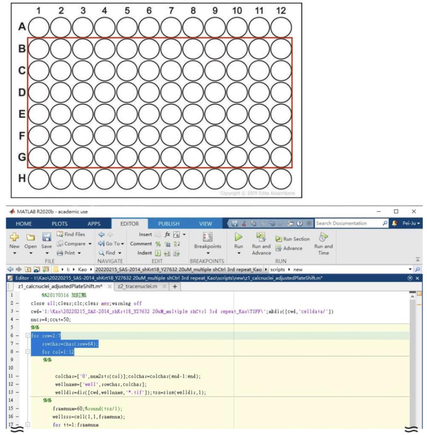
  Figure 3. Example of a 96-well plate setting corresponding to the row and column number in Z1_calcnuclei_adjustedPlateShift
  
  This script defines nucleus based on a modified threshold selection method. By measuring fluorescence signals (DAPI; Channel 1) to define centroid of every nucleus, we can acquire the location information of each cell from all the acquired images. This allows users to get all the information of cell location.
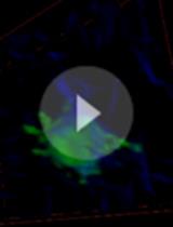
  We first retrieved the centroid of each cell for further calculation of cell movement. The highest signal in the DAPI channel within an estimated distance would be seen as cell centroids, and we labeled these signals as red dots in the image (Figure 4, left panel). To confirm the nucleus definition correctness, we examine the overlap of red dots and green dots (nuclei mask) in the representative figure (Figure 4, right panel). The original Hoechst signal is labeled as red, and our nuclei mask is labeled as green. The nuclei mask is based on Hoechst signal with extra restrictions on size and shape to eliminate noise (such as cell debris) from our analysis. The higher the overlapped ratio of red and green dots, the higher the precision of recognizing the cells. Then, we compare the images between centroids and nuclei masks to double-check if our centroids are in the right place.
  
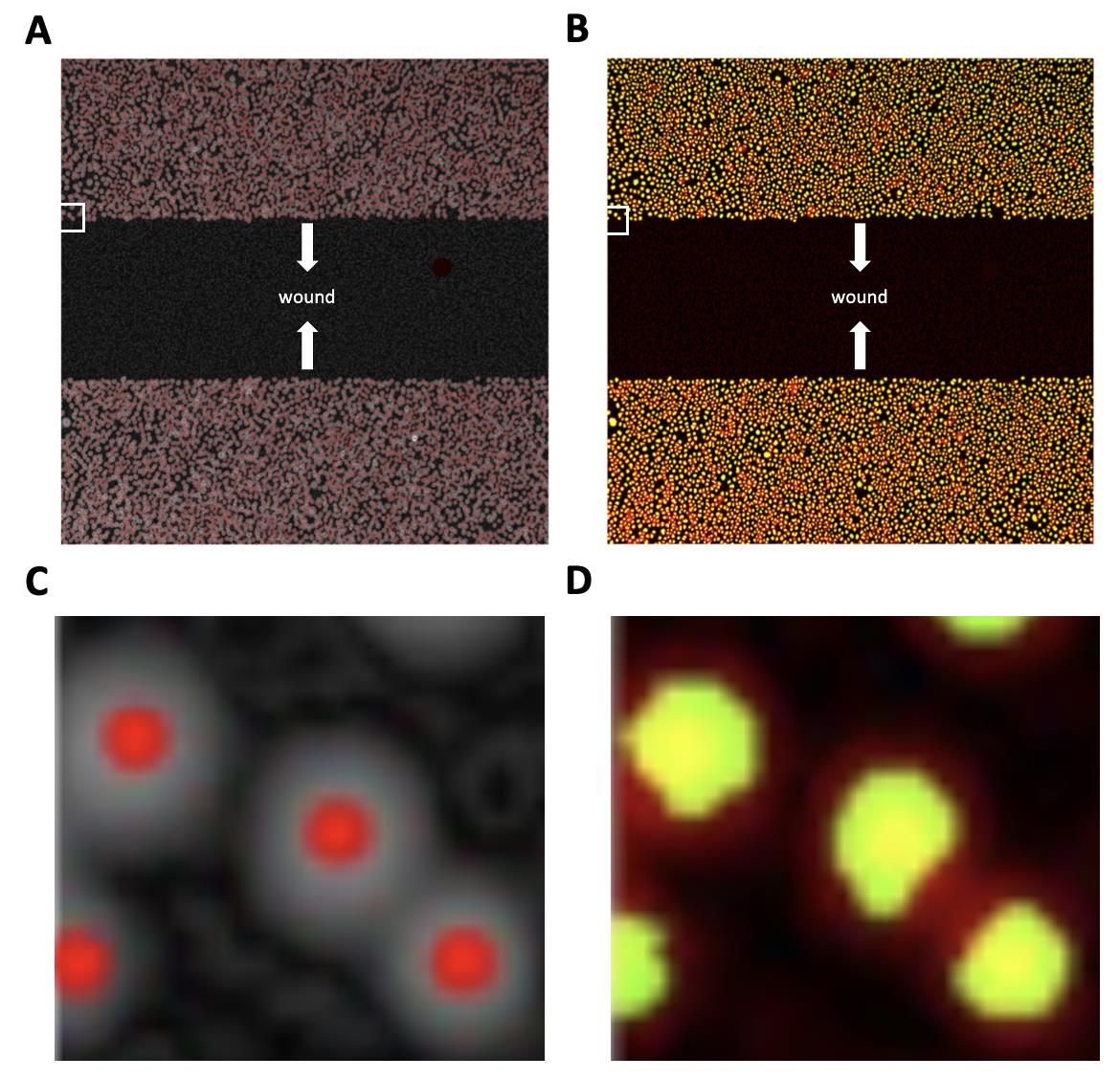
  Figure 4. Example of capturing cell nuclei after running Z1_calcnuclei_adjustedPlateShift. (A) The red dots are the highest Hoechst signal compared with its surrounding signal as our centroids; this labeled centroid area is magnified in (C). (B) Overlap of the image in the panel with the nuclei mask (green) generated by the processed Hoechst signal and the original Hoechst signal (red), which is magnified in (D). The white arrows in (A) and (B) indicate the direction of cell migration, and the white squares are the cells chosen for magnification.

Monitoring cell movement: Z2_trace nuclei
This script calculates changes of cell location between each time frame.
1. Open Z2_trace nuclei.m.
2. Change the file path in line 3 and fill in the row and column number based on your experimental setting in line 7 and 9 (Figure 5).
3. (Optional) Change the nuclear size (line 4). The nucleus size should be changed based on your cell line (in this case, we use 4 for SAS to best discriminate each cell).
4. Click Run.
  
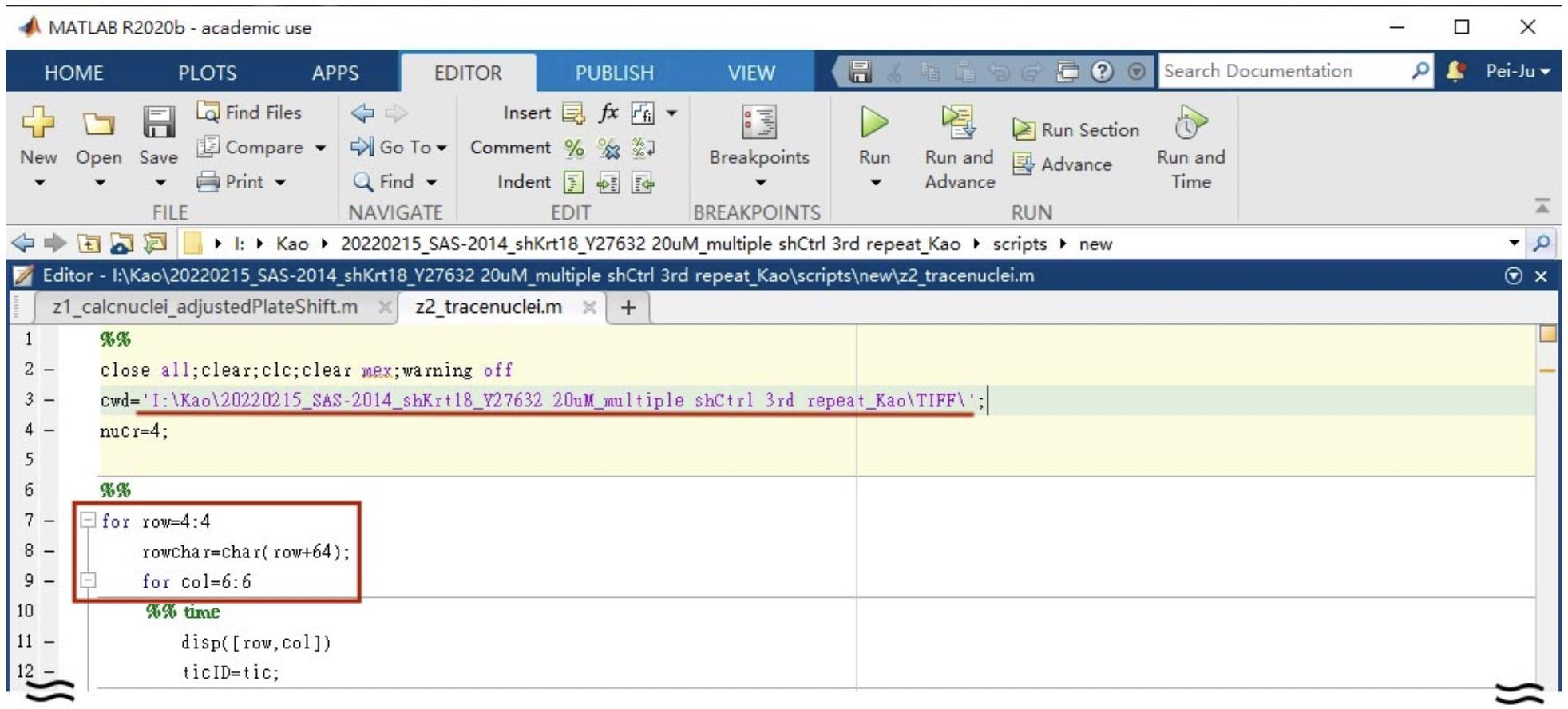
  Figure 5. Screenshot of the Z2_trace nuclei user interface. The underlined and circled areas need to be adjusted in each experiment.

Get cell information: Z3_getcellparameters062945

Parameters such as speed, coordination, and directionality were analyzed using MATLAB.

Open Z3_getcellparameters062945.m.
Change the file path in line 3 and fill the row and column number based on your experimental setting in line 7 and 9 (Figure 6A).
(Optional) Change the nuclear size in line 4. The nucleus size should be changed based on your cell line (in this case, we use 4 for SAS to best discriminate each cell).
Click Run.

Define the number of analyzed cells:

Fill out the cell number in line 16 that you would like to analyze (Figure 6A). Selected cells should be marked as red. Below is an example of analyzing 1,000 and 10,000 cells (Figure 6B). Note that for random migration, we select all the cells in the frame.

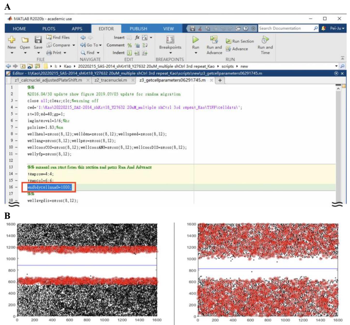
Figure 6. Example of different parameter settings for cell numbers used for migration analysis. (A) User interface of Z3_getcellparameters062945. The circled area defines the number of cells being analyzed in tracking. (B) The left panel shows the analysis of 1,000 cells, and the right panel shows the analysis of 10,000 cells. The black dots represent the cells in the entire image, and the red dots represent the cells going to be analyzed. We also show the XY axis from 0 to 1,600 to better spot the exact cell location from the figure and exported data.

Data will be saved under the file called cell data. File name: Well name + bestsp.

Parameters will be saved into several spreadsheets (Figures 7 and 8, Table 1); each spreadsheet is a parameter of migration behavior. An example of exported data is shown in Figure 8. Note that the angle data (wellang) need to be further calculated through the formula: π/2 - θ. θ is the original value shown on the spreadsheet.

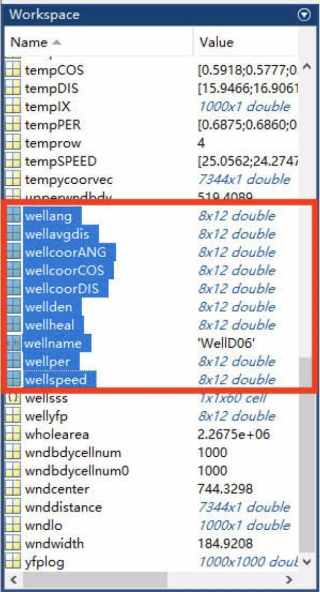
Figure 7. Screenshot of Z3_getcellparameters062945 in workspace after running this script. MATLAB files have been generated after running Z3_getcellparameters062945, and the circled files are exported to Excel for further analysis.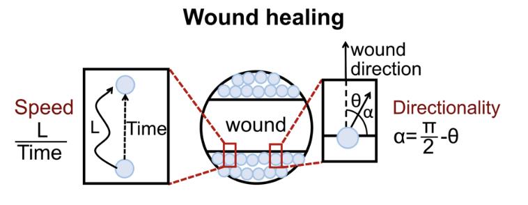

Figure 8. Graphical schematic of variables used in cell migration analysis. The directionality is the angle of cell movement relative to the wound direction. Retrieved from Yu et al. (2021).

Table 1. Migration statistics

Variable	Calculation	Description
Wellang	π/2-α	Average angle of cell movement relative to the wound direction in the well
wellcoorCos	Cos θ	Average cell–cell coordination in the well
wellden	Total cell number in each frame	Cell number of this frame. Note that cell migration speed could be influenced by cell density, so this data has to be quite consistent among each well
wellspeed	Distance/time	Average cell migration speed in the well. The unit is μm/h.
wellper	Displacement/distance	Average consistency of directionality of the cell movement in the well

To make the definition clear, Figure 7 explains the variables being used.

Although our scripts generate all variables, we use different parameters for analyzing different cell migrations. For wound healing assay, we analyzed the speed, angle, coordination, and persistence of cell migration. However, we do not analyze cell angles for random migration because we define cell angle as how cells deviate from the direction of the wound. Here, we provide an example of the data we used for analyzing the wound healing assay result (Figure 9).

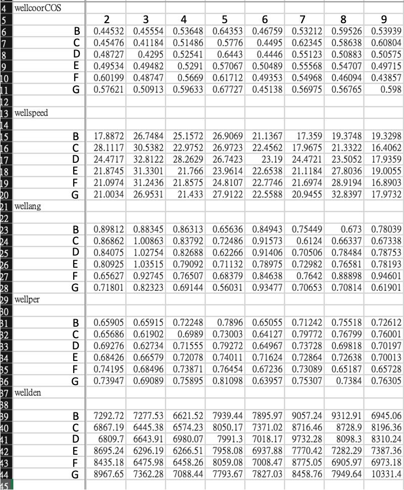
Figure 9. xample of the population of cell data. Each data point corresponds to the mean value of each well. These data are from row B–G, column 2–9 of a 96-well plate.

These data could be plotted into bar graphs for visualization (Figure 10).

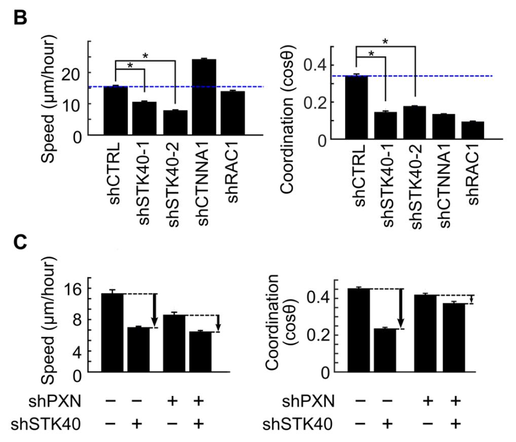
Figure 10. Example of the bar graph for cell migration analysis. Retrieved from Yu et al. (2021).

Validation of protocol

This protocol or parts of it has been used and validated in the following research article(s):

Yu et al. (2021). Synthetic dysmobility screen unveils an integrated STK40-YAP-MAPK system driving cell migration. Sci. Adv. 7(31): eabg2106 (Figure 1, panel C and G, and Figure 2, panel B and C).

Acknowledgments

Funding: This work was supported by grants from The Ministry of Science and Technology in Taiwan (MOST 107-2320-B-002-038-MY3 and MOST 108-2926-I-002-002-MY4), National Taiwan University Hospital (NTUH 106-T02, NTUH 107-T13, NTUH 108-T13, and VN 109-14), and The Liver Disease Prevention and Treatment Research Foundation in Taiwan. This protocol was adapted from Yu et al. (2021).

Competing interests

The authors declare that they have no competing interests.

References

Friedl, P. and Gilmour, D. (2009). Collective cell migration in morphogenesis, regeneration and cancer. Nat. Rev. Mol. Cell Biol. 10(7): 445–457.
Jin, W., Shah, E. T., Penington, C. J., McCue, S. W., Chopin, L. K. and Simpson, M. J. (2016). Reproducibility of scratch assays is affected by the initial degree of confluence: Experiments, modelling and model selection. J. Theor. Biol. 390: 136–145.
Luster, A. D., Alon, R. and von Andrian, U. H. (2005). Immune cell migration in inflammation: present and future therapeutic targets. Nat. Immunol. 6(12): 1182–1190.
Weijer, C. J. (2009). Collective cell migration in development. J. Cell Sci. 122(18): 3215–3223.
Yu, L. Y., Tseng, T. J., Lin, H. C., Hsu, C. L., Lu, T. X., Tsai, C. J., Lin, Y. C., Chu, I., Peng, C. T., Chen, H. J., et al. (2021). Synthetic dysmobility screen unveils an integrated STK40-YAP-MAPK system driving cell migration. Sci. Adv. 7(31): eabg2106.

Supplementary information

The following supporting information can be downloaded here:

Z1_calcnuclei_adjustedPlateShift.m
Z2_trace nuclei.m
Z3_getcellparameters062945.m