- Protocols

- Articles and Issues
- For Authors
- About
- Become a Reviewer

Quantitative Live Confocal Imaging in Aquilegia Floral Meristems
(*contributed equally to this work) Published: Vol 12, Iss 12, Jun 20, 2022 DOI: 10.21769/BioProtoc.4449 Views: 3626
Reviewed by: Vivien Jane Coulson-ThomasBeatriz GoncalvesAnonymous reviewer(s)
Original research article
The authors used this protocol in:
Feb 2022
Advertisement


Protocol Collections
Comprehensive collections of detailed, peer-reviewed protocols focusing on specific topics


Abstract
In this study, we present a detailed protocol for live imaging and quantitative analysis of floral meristem development in Aquilegia coerulea, a member of the buttercup family (Ranunculaceae). Using confocal microscopy and the image analysis software MorphoGraphX, we were able to examine the cellular growth dynamics during floral organ primordia initiation, and the transition from floral meristem proliferation to termination. This protocol provides a powerful tool to study the development of the meristem and floral organ primordia, and should be easily adaptable to many plant lineages, including other emerging model systems. It will allow researchers to explore questions outside the scope of common model systems.
Keywords: Live imagingBackground
Meristems are groups of pluripotent stem cells, typically located at the tips of shoots (Steeves and Sussex, 1989). Many fundamental features of meristems are shared across all vascular plants, e.g., the maintenance of a pool of undifferentiated cells, regulated cell proliferation and expansion, and control of post-embryonic organogenesis. However, there remains a great deal of unexplored variation in meristem structure and behavior across land plants. Exploring this diversity is hampered by the reliance on common developmental techniques, such as fixed tissue sectioning and imaging, that do not allow processes such as spatial and temporal patterns of cell division and expansion to be directly observed. In model systems such as Arabidopsis thaliana, genetic and molecular tools have been coupled with advancements in live imaging techniques to allow analyses of both cell behaviors and gene expression in real time. These tools have provided considerable progress in our understanding of meristem development (e.g., Prunet et al., 2016; Geng and Zhou, 2019; Shi et al., 2020; Caggiano et al., 2021; Silveira et al., 2022). However, these advancements are currently limited to a small number of model species, and there is a pressing need to develop quantitative live imaging techniques in non-model systems, and specifically, approaches that may be broadly practical across a range of plant taxa. Here, we present a detailed protocol for live imaging and analysis of floral meristems in Aquilegia coerulea, a member of the buttercup family (Ranunculaceae). This protocol provides a powerful tool to study the development of the meristem and initiation of floral organs, and should be easily adaptable to many plant lineages, including other emerging model systems. This protocol will allow researchers to explore questions outside the scope of common model systems.
Materials and Reagents
35 × 10 mm Petri dish (Corning, product number: 430588)
100 × 15 mm Petri dish (Fisher Scientific, catalog number: FB0875712)
1.5 mL microcentrifuge Eppendorf tubes
Parafilm
Kimwipe
Microscope slides (no special coating required)
Aluminum foil
128 cell plug trays and 4-inch plant plots
Seeds of Aquilegia × coerulea ‘Kiragami’ can be purchased from Swallowtail Garden Seeds (Santa Rosa, CA, USA)
Agar (Invitrogen, catalog number: 16500-100)
Linsmaier & Skoog medium (Caisson Labs, catalog number: L2P03)
Sucrose (Macron Fine Chemicals, catalog number: 57-50-1)
NaOH (Sigma-Aldrich, catalog number: 221465)
Kinetin (Sigma, catalog number: K0753-1G)
Gibberellic Acid (Sigma, catalog number: G7645-1G)
100% EtOH
Sterile ddH2O
Bleach
Propidium Iodide (Sigma-Aldrich, catalog number: P4864)
Note: Potential carcinogen; avoid contact with skin and eyes; wear suitable protective clothing, gloves, and eye/face protection.
Glue (any type of glue that can glue Petri dish to the glass slides)
Culture medium (see Recipes)
Equipment
Scalpel with No. 10 blade (BioQuip Products, catalog number: 2723A)
Straight dissecting needle (Carolina, catalog number: 627201)
Precision Watchmaker's Forceps, Extra-Fine Point (Carolina, catalog number: 624791)
0.5 mm Glass beads (Sigma-Aldrich, catalog number: 18406)
Razor blades
Microscope (Zeiss Stemi DV4 Stereo)
Microscope (LSM 980 NLO Multi-photon with a water immersion lens W Plan-Apochromat 20×/1.0 DIC UV-IR M27 75mm)
Software
FIJI (https://imagej.net/software/fiji/) or ImageJ (https://imagej.net/software/imagej/)
MorphographX (MGX) https://morphographx.org/software/.
Procedure
Plant materials and growth conditions
Seeds of Aquilegia × coerulea ‘Kiragami’ can be purchased from Swallowtail Garden Seeds (Santa Rosa, CA, USA), and germinated in wet soil in plug trays, which generally takes two to three weeks.
When the seedlings develop their first two true leaves, they are transplanted from plug trays to five-inch pots. Seedlings and young plants are grown in growth chambers with 16-h daylight at 18°C, 8-h dark at 13°C, and humidity under 40%. In these regular growth conditions, the plants are watered twice per week.
Once the plants develop five to six true leaves, they are transferred into the vernalization chamber, which is set at 16-h daylight at 6°C, and 8-h dark at 6°C. They should be well watered (i.e., the soil is fully hydrated) before being moved into cold conditions, and are generally not watered during the vernalization period.
Plants stay in vernalization for three to four weeks, and are then moved back into regular growth chambers for flowering. We usually put a small amount of controlled-release fertilizer in each pot post vernalization. Generally, inflorescences start to develop three weeks after vernalization.
Dead leaves should be actively removed, to prevent fungal or pest infections.
Preparation of culture/imaging plates
Take an empty 1,000 μL pipette rack and gently press the foil square into each one of the rack holes, to create a round well (Figure 1a, b). Cut small squares of aluminum foil (1 × 1 cm). Carefully store foil squares in an autoclavable container (such as a glass Petri dish) and autoclave (Figure 1c).
Autoclave glass beads and ddH2O.
Prepare the culture media according to Recipe 1.
While still molten, fill the 35 × 10 mm Petri dishes half way with agar, quickly place one foil square in the center of the Petri dish, concave side up. With sterile tweezers, place a glass bead into the depression in the foil square (Figure 1). This is sufficient to ensure that the convex side of the foil is pressing into the agar. Once the bead is on the foil square, the foil will automatically gravitate to the center of the plate. Let the plates cool and solidify inside the sterile hood. Once solid, using tweezers, remove the glass beads and carefully peel off the foil square. This leaves a shallow well in the agar for mounting the meristems.
Solidified plates can be stored at 4°C for 2 months.
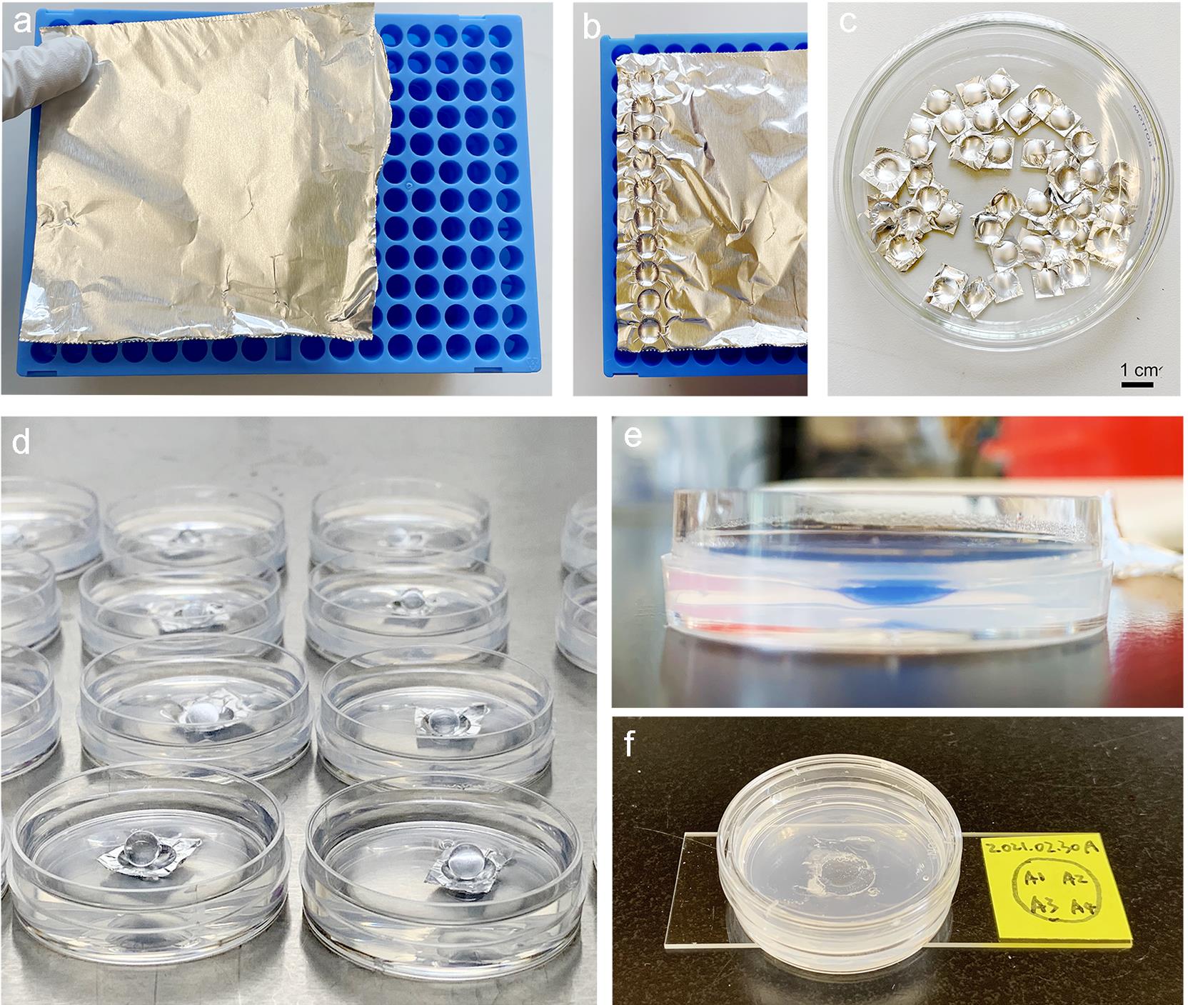
Figure 1. Making plates for live imaging. (a) Take an empty 1,000 μL pipette rack and gently press the foil square into each one of the rack holes, to create a round well. (b) A strip of wells. (c) Foil squares are autoclaved and stored in a glass Petri dish. (d) Examples of plates solidifying in a sterile hood with foil squares and glass beads in place. (e) A 35 × 10 mm Petri dish with blue dye to show the well in the center, where the meristems will be positioned. (f) The 35 × 10 mm Petri dish will then be glued onto a microscope slide. The slide is labeled with dates, and A1–A4 are the meristem label and their relative locations in the well.
Tissue dissection and mounting
The forceps, surgical needles, and dissection blades are all sterilized in 10% bleach, washed in ddH2O, and dried with Kimwipes before dissection.
Young axillary inflorescences or whole inflorescences are excised off the plant using forceps or scissors, for meristem dissections (Figure 2).
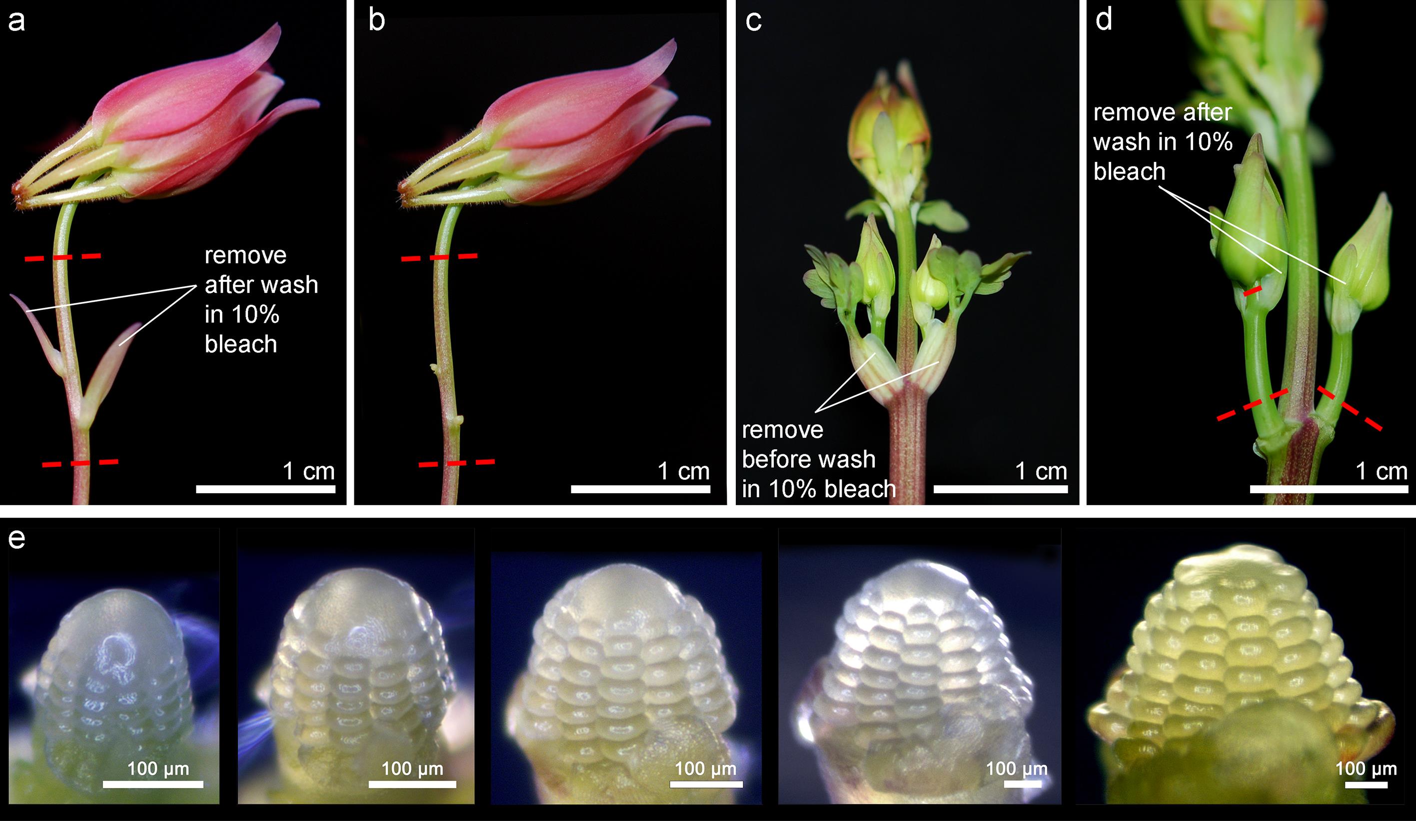
Figure 2. Developmental stages for dissecting FMs for imaging. Axillary meristems can be obtained from either a lateral inflorescence branch (a, b) or a young inflorescence (c, d). Leaves that should be removed before or after the 10% bleach wash are indicated. Red dash lines indicate the locations where the floral axis will be excised for the bleach wash. (e) Example of a FM undergoing the stages from continuously producing more whorls of floral organs to the early developmental phase of carpels. This FM was imaged every two days.Inflorescences are washed in freshly prepared 10% bleach in a 100 × 15 mm Petri dish for 20 min. Any leaves and bracts on the stem should be removed using the forceps, but the attachment points of the petioles should be left on the stem (Figure 2); if the petiole is completely removed from the stem, we found that the bleach solution will enter the wound and spread through the cells quickly, which kills the axillary meristems as well.
The stems are then washed with double-distilled water (ddH2O) three times in the same 100 × 15 mm Petri dish, to completely remove the bleach residue, after which the stems are kept immersed in sterile ddH2O.
When dissecting, put one stem under the microscope (the rest remaining in distilled water), and carefully remove the bracts and sepals of each floral meristem, using the tip of a dissecting needle. Then, excise the meristem off the branch with the scalpel, and transfer it onto a 35 × 10 mm Petri dish with the culture medium. Ensure the base of the stem (usually there is about 1 mm of stem remaining) holding the meristem is pushed into the agar. We typically mount four floral meristems per dish.
Glue the Petri dish to a microscope slide, and label the date and the meristems on the slide (Figure 1c).
Staining
Meristems should be stained for 1–3 min in the Petri dish, by applying 50 μL propidium iodide (0.5 mg/mL) directly to the meristems, to ensure the meristems are fully immersed. The mounting well should sufficiently contain the stain, so that it creates a dome over the meristems. Take care of there being sufficient stain, so that the meristems are fully immersed in stain throughout the whole staining period. It is important to note that the staining time will likely be specific to the plant and tissue being imaged, so here we just give a general time range; it is recommended that the staining time be optimized for each experiment. We would recommend starting with a low concentration for 1 min, and adding time only if the tissue seems under-stained. Another important optimization is the staining for subsequent imaging time points. Aquilegia meristems were stained for 2.5 min for time point 1, then 2 min for time points 2 and 3, and 2–3 min for time-point 4.
Carefully pipette off the stain, and wash the meristems by pipetting with ddH2O three times.
Imaging
Note: Imaging will differ depending on the type of confocal and objective lenses available, as well as the type of tissue or stain used.
Meristems were imaged immediately after staining, using a LSM 980 NLO Multi-photon confocal laser scanning microscope (Ziess, Germany) equipped with a water immersion objective (W Plan-Apochromat 20×/1.0 DIC UV-IR M27 75mm, Ziess).
The Petri dishes were filled with ddH2O while imaging, and the water was immediately removed after imaging.
A DPSS 514nm laser was used for excitation, and emission was collected between 580–670nm.
Scans were frame averaged 2× and z-sections taken at 2-µm intervals. This interval will vary depending on the size of the tissue, and we found that 2 µm was sufficient for downstream analysis, while also minimizing the time the tissue was subjected to the laser. On average, it takes 2 min to image a young Aquilegia FM, and about 4 min to image a young Aquilegia bud with early carpel development.
After imaging, the remaining water in the Petri dishes was carefully removed by pipetting using a P20 pipette, and the Petri dishes were returned to the tissue culture growth chamber.
Samples were imaged every 48 h, typically for 3–5 time-points.
Image processing
Note: The following protocol for conducting segmentation and lineage tracing of the confocal images was adapted from (de Reuille et al., 2014; Strauss et al., 2019), and the user manual at https://www.mpipz.mpg.de/MorphoGraphX/help, all of which detailed the structure of MorphoGraphX (MGX), including how the image data are stored, extracted, and processed. Here, we focus on the steps and parameters that are specific to processing confocal images of Aquilegia floral meristems, and steps to reproduce figures in Min et al. (2022). We will use two original .czi files from our study as an example, which can be downloaded from this google drive link: https://drive.google.com/drive/folders/1WjaCieLGrnTW7d51143b8HOn-dYmsMU-?usp=sharing Images of individual time points will be processed separately first, then loaded together for lineage tracing (details in the following section Parent Labeling & Lineage Tracing).
Software installation and equipment setup
Download the newest version of MGX from https://morphographx.org/software/. Since the software improvements have mostly been implemented in the Linux versions, installation of the Linux operating system is preferred. To run, MGX requires a computer nVIDIA graphics card that supports CUDA, with at least 2 Gb of video memory and 8 Gb of the main memory of the computer itself. A larger video memory, a larger main computer memory, and/or a multi-core CPU can significantly shorten the processing time for some of the steps.
Processing a large amount of imaging data with MGX can be time-consuming, and we strongly recommend readers have a comfortable workstation with proper office ergonomics if possible. An ultrawide monitor, or a dual-monitor setup, can be extremely helpful, especially during the parental lineage tracing error correction process.
Load image into MorphoGraphX
Convert the format of the stack image: Open the stack image (e.g., the 20210207_r8_A1.czi files) with FIJI (https://imagej.net/Fiji) or ImageJ: (https://imagej.net/Welcome), adjust the brightness and contrast, and save the image as 20210207_r8_A1.tif format.
Note: The images we acquired from the confocal microscope can be dim because we wanted to minimize tissue damage from both laser power and laser exposure time (which, in turn, slows down the growth), and thus the adjustment in brightness and contrast was almost always needed. Images that look slightly over-saturated in FIJI/ImageJ after adjusting for brightness and contrast, look better when loaded in MGX (Figure 3).
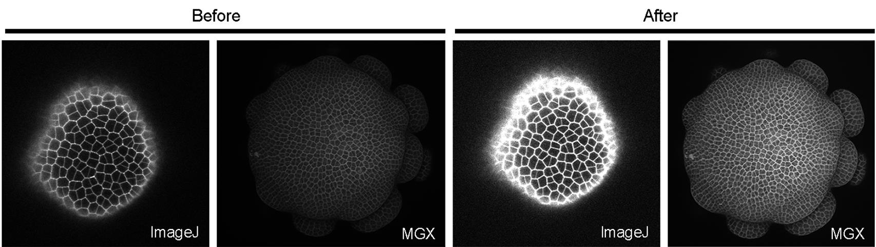
Figure 3. Comparison of how a confocal stack looks in ImageJ and MGX before and after adjusting the brightness and contrast. Images that appear to be slightly over-saturated in ImageJ generally look good in MGX.Load the stack into MorphoGraphX: either drag the 20210207_r8_A1.tif file directly onto the MGX interface (Figure 4), or Stack1 → open → choose the image.
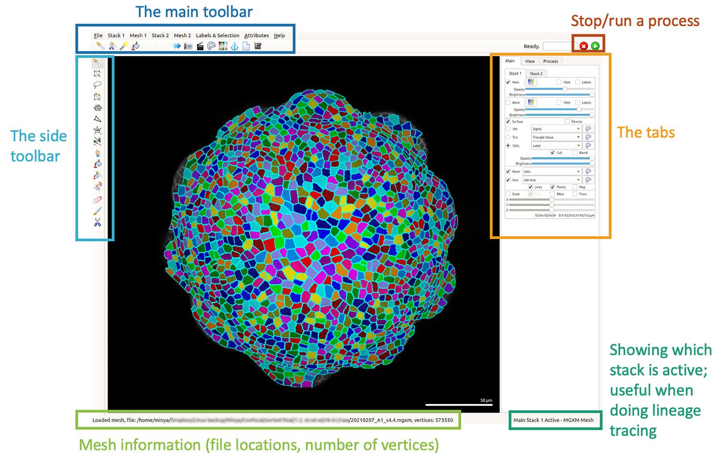
Figure 4. Overall layout of MorphgraphX interface.If the stack still appears to be dark, there are two ways to directly adjust the brightness in MGX, instead of adjusting the brightness/contrast in Fiji, and loading the stacks again: 1) under the Main tab, under Work, change Opacity; 2) go to the View tab, and change the brightness and contrast under View Quality.
You can rotate the stack by using the left click of your mouse, move the stack to different parts of the screen with the right-click, and zoom in and out with the scroll wheel. By default, Stack 1 will appear green, and Stack 2 will be red; the setting of the colors can be changed using the Main Stack Colormap, under the Main tab
 .
.
Extract the surface
Go to tab, Process → Stack → Filters → Gaussian Blur Stack; change all the X/Y/Z Sigma parameters (appears at the right bottom corner; double click the cell to change) to 1; run the process twice (either by double-clicking the processor, or hitting the “Run” arrow
 on the upper right corner).
Note: It is important to blur each stack the same number of times, especially when dealing with images for lineage tracing.
Run Process → Morphology → Edge Detect, which creates a solid global shape of the object.
Optional: Remove unwanted parts. For example, if we only want the top part of the meristem, we could remove the extra stamen/staminode primordia by clicking on “Voxel Edit
 ” on the top bar; Press Alt-key and left click the mouse, to erase parts that you don’t want.
Note: 1) If the Alt-key is not working, it is likely due to a conflict in the hotkey setting in your operating system, which already assigned a function to the Alt-key, and thus prevents it from being used for selection in MorphoGraphX. You can change this setting in your operating system by assigning other keys to avoid the conflict. 2) Removing unwanted parts using the voxel edit can increase the speed of downstream processes, but the removal of parts is not reversible, so this step is generally not recommended unless there is a significant constraint on computer capacity.
Optional: If there are holes on the shape, run Stack → Morphology → Fill Holes. Skip if no hole is observed.
Note: The adjustable parameters in this step are the X/Y-Radius. The bigger they are, the more likely they can fill the holes. However, the bigger they are, the more possible it is going to change your surface shape.
Go to Mesh → Creation → Marching Cubes Surface, change the threshold parameter to 20,000, run the process.
Trim off the bottom. In the Main tab, ensure that the Mesh checkbox and “View” option are set to “All”. This will enable the visualization of the mesh. Click the “Select points in mesh (Alt+V)
 ” tool on the left toolbar, and hold the Alt-key to select the bottom vertices of the apex. The selected vertices should turn red. Hit the delete key on the keyboard to remove them. To make this easier, it is better to have the apex in a horizontal position. You can do this by left-double clicking on it. Try to delete the bottom cleanly. Save the mesh as “20210207_r8_A1_s.c6.mgxm”.
Note: Since many meshes will be saved during the process, we tried to name the files in a clear way, so that one can easily recognize that a given mesh is produced by a specific step. In this example, the information is recorded as “s.c6”: s stands for single time point and c6 refers to step 6 of part C “Extract the surface” of this protocol.
Run Mesh → Structure → Subdivide. Then go to Mesh → Structure → Smooth Mesh, change the Passes number to 10 (the default is 1), and run the process. Repeat this subdivide step and then smooth the process twice more (i.e., three times in total). By now, the total number of vertices (shown in the bottom left window) in the mesh for an early stage FM should be above 500,000, while for an older stage FM should be approximately 1,000,000.
Note: Each subdivision increases the total number of vertices by approximately four-fold. The last round of subdividing and smoothing can be demanding on computational power. The vertices look like little triangles when magnified.
Save the mesh as “20210207_r8_A1_s.c8.mgxm”.
Go to the Main tab, Unselect “Mesh”. Make sure “Main” and “Surf” are selected, but “Work” is not. Then run Process → Mesh → Signal → Project Signal, to project the signals to the surface.
Note: The default Max Dist (µm): 6.0 is good for Aquilegia floral meristems, since they have relatively large cells, especially when compared to Arabidopsis meristem cells. If visualizing a tissue with smaller cells, the Max Dist can be decreased accordingly.
Save the mesh as “20210207_r8_A1_s.c10.mgxm”.
Cell segmentation
Go to Process → Mesh → Segmentation → Auto-segmentation and change the following parameters from default: normalize to “No”, auto-seeding to 3.0, blur cell radius to 3.0, combine to 1.1. Run the process.
Note: The auto-segmentation process can be demanding on the computational power. For Aquilegia floral meristems, depending on the developmental stages, we obtained good results by changing the auto-seeding and blur cell radius to 2.0, 2.5, or 3.0. The radius for auto-seeding and blur cells should be the same.
Save the mesh as “20210207_r8_A1_s.d2.mgxm”.
Correct segmentation errors
No matter how good the image stack is, there are likely to be segmentation errors, especially with samples such as Aquilegia floral meristems, that contain hundreds to thousands of cells in a stack. It is very important to correct as many errors as possible at this step, since it will greatly reduce the time that will likely be needed in future processes to correct parental labeling errors (which is relatively more time-consuming compared to correcting segmentation errors). It is also important to constantly save the newer version of the mesh (e.g., 20210207_r8_A1_s.e0.mgxm). The two processes with opposite functions, “Watershed Segmentation” and “Segmentation Clear”, are located right next to each other on the list, and it is not impossible to click the wrong button during processing. If the “Segmentation Clear” is run by accident on the whole mesh, while the newest version of the corrected mesh has not been saved, it means starting over again.
Checking segmentation errors can be done by zooming in on one part of the mesh and selecting “Vtx” under the Surface panel of the Main tab, and then accessing the Mesh panel under the “Cells” option. By toggling back and forth between the checked and unchecked options in the Mesh checkbox, you can compare the cell wall positions and segment boundaries. Correct all the possible errors in that region, then move to another part of the mesh, and repeat the process. There are a few types of common segmentation errors (Figures 5–7):
If a cell is over-segmented: If cell A is over-segmented into A1 and A2, select “Add label to selection
 ” on the left toolbar, press Alt-key, and click on A1 (or A2). Then select “Fill label (Alt+M)
 ” on the left toolbar, press Alt-key, and click on A2 (or A1) (Figure 5).
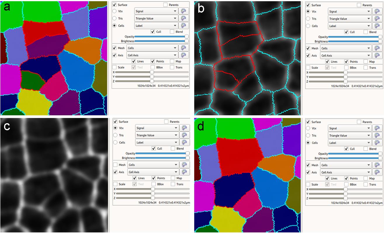
Figure 5. Examples of over-segmented cells. (a) How over-segmented cells (outlined in red) look under the Surface/Cells view. (b) How over-segmented cells (outlined in red) look under the Surface/Vtx view. (c) How the mesh looks. Over-segmented cells can be easily spotted by comparing between (c) and (b). (d) How cells look after over-segmentation has been corrected.If a cell is under-segmented: This is a relatively common situation for cells at the boundary of the stack (due to faint signals), and at the organ boundaries (because the cells at the boundary are much smaller than the auto-segmentation radius). Click “Select points in mesh (Alt+V)
” on the left toolbar, press Alt-Key, and select parts of the cell that need to be corrected (as long as some vertices in that cell were selected, it is fine). Then, under the Process tab, run Mesh → Selection → Extend to Whole Cells, which selects all the vertices in that target cell (Figure 6). On the left toolbar, click on “Erase selected ” to remove the labels from the cell. Labels can also be removed by running Mesh → Segmentation → Segmentation Clear under the same Process tab (Figure 6). Then choose “Add new seed (Alt+B)
 ” from the left toolbar, press the Alt-key and the left click of the mouse, to draw the outlines of the cells (Figure 6). Theoretically, the cells can be segmented as long as there is at least one seed inside, but drawing out the rough outlines of the cells can help with correct segmentation, because sometimes the cell boundaries are faint. Lastly, under the Process tab, run Mesh → Segmentation → Watershed Segmentation (Figure 6).
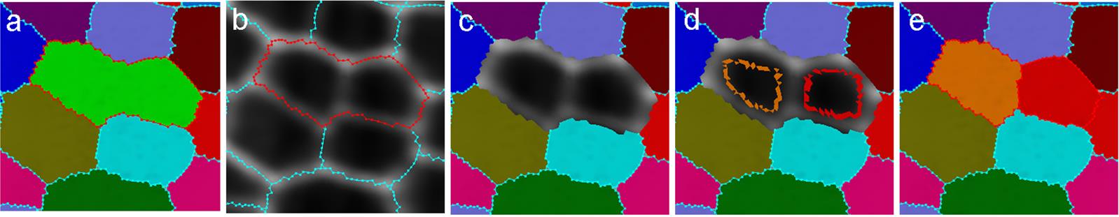
Figure 6. Examples of under-segmented cells. (a) An under-segmented cell outlined in red. (b) Under-segmented cells can be easily spotted by comparing the segmented outlines to the original mesh. (c) The label of the under-segmented cell being cleared. (d) The two cells being re-seeded. (e) How the labels look after the under-segmentation is corrected.If the boundary of a cell is incorrect: This is most likely due to a faint signal in the cell wall staining (Figure 7). On the left toolbar, click “Add label to selection
 ”, then press the Alt-key, and click the cell that needs to be corrected. Then choose “Add current seed (Alt+N)
 ” from the left toolbar, use the left click of the mouse to fill in the gaps, and draw the correct boundary (Figure 7). Then, under the Process tab, run Mesh → Segmentation → Watershed Segmentation (Figure 7).
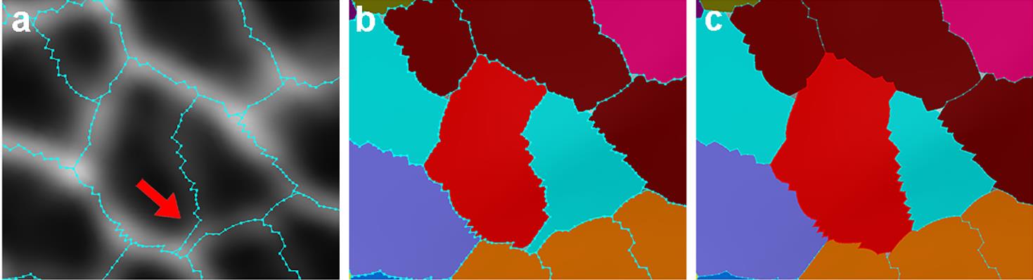
Figure 7. Example of a cell with incorrect boundary. (a) Red arrow pointing to the incorrect boundary of a cell. (b) How the original segmentation looked. (c) How the corrected segmentation looked.Remove the cells on the boundary of the mesh: After all visible errors are corrected on the mesh, run Mesh → Cell Mesh → Fix Corners Classic, under the Process tab. Then click “Select points in mesh (Alt+V)
 ” on the left toolbar, press Alt-key, and select cells on the boundary of the mesh. Then, under the Process tab, run Mesh →selection → Extend to whole cells. After the cells are selected, click “Delete selected” on the left toolbar, and save the mesh as “20210207_r8_A1_s.e4.mgxm”.
This last step is important because the sizes of the cells on the boundary are likely to be inaccurate due to several reasons: 1) the confocal Z-stack may have stopped scanning at this point, without including the entire cell on the boundary; and 2) we arbitrarily trimmed off the bottom of the stack in step C6, which may have trimmed off parts of cells located on the boundary (Figure 8).
After the first layer of cells on the boundary is removed, run Mesh → Cell Mesh → Fix Corners Classic, under the Process tab again, and save the mesh again. This will be the mesh (i.e., 20210207_r8_A1_s.e4.mgxm) that is used to conduct lineage tracing.
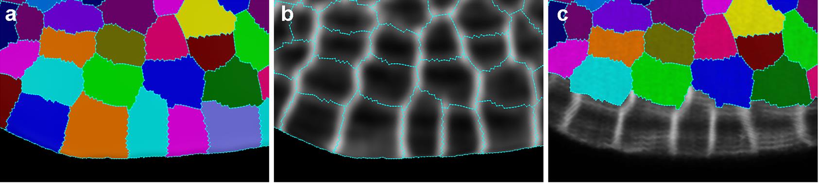
Figure 8. Removing cells on the boundary of the mesh. (a, b) How the labels look before removing the cells on the boundary, which had unnatural shapes. (c) How the labels looked after removing the cells on the boundary.Parent labeling & Lineage tracing
After processing the stacks and meshes from both time-point 1 (20210207_r8_A1_s.e4.mgxm) and time-point 2 (20210209_r8_A1_s.e4.mgxm), they are ready to conduct parental labeling and lineage tracing.
Parental labeling
Go to the Main toolbar, load the segmented mesh for time point 1 on Mesh 1, and the segmented mesh for time point 2 on Mesh 2. Both meshes are now loaded as meshes of Stacks 1 and 2 under the Main tab, respectively. The main stacks (i.e., the original .tif files) can also be loaded using the Main toolbar for Stacks 1 and 2. It is a personal preference whether or not to load the main stacks, because they are not required for the lineage tracing process, but it might look nicer to have the main stack shown when taking pictures.
Go to the View tab, and check “Stack1” in the Control-Key-Interaction panel. This allows you to move the meshes separately. Using the right click of the mouse alone will move both meshes together, but using the right click of the mouse while pressing the Control-key on the keyboard will only move Stack 1. Use the control key and the mouse to move Stacks 1 and 2 side by side on the screen.
Go to the Main tab Stack 1, next to the Mesh checkbox, click Colors Editor
 to change the colors of Mesh 1 and/or Mesh 2, so that they are different from each other.
Go to the Main tab Stack 1, make sure the checkboxes of Main, Work, and Surface panels are all unchecked, but the one for Mesh is checked. Make sure that “Cells” is selected as the view option for both the Mesh and the Surface panels, and the view option for Cells is selected as “Label”.
Go to the Main tab Stack 2, uncheck Main and Work, but check Surface and Mesh. The view options for Surface and Mesh should be “Label” and “Cells” as well, respectively. Then check the checkbox of Parents to the right of the Surface checkbox. The colored segmented cells in Stack 2 should disappear after this.
When the meshes of the meristems are first loaded, we see the front view of the meristems. Use the left click on the mouse and the Control key to adjust the orientations of both meshes, so that the side views are shown.
Use the left click of the mouse and the Control key to move Mesh 1 above Mesh 2. Then, use the left click of the mouse alone to rotate both meshes, so that the front views are shown again.
Look for a few cells on Meshes 1 and 2 that appear to be the same. Usually, the large cells at the center of the meristems are the most easily recognizable. Transfer Mesh 1 on top of Mesh 2, by pressing the Control-key and using the right click of the mouse to match those recognized cells on both meshes.
Adjust the orientation and angles of Mesh 1 using the left click of the mouse and the Control-key, to make more cells on both meshes overlap. If the growth between the two time points is rather large, adjust the size of Mesh 1 by going to the Main tab Stack 1, check the Scale checkbox, and increase the X values (adjusting Y or Z is also fine, since all axes are linked).
To transfer labels from Mesh 1 to Mesh 2, go to the Main tab Stack 2, so that Stack 2 is active. Select “Grab Label
 ” from the left toolbar, hold the Alt-key, and click on the cells that are aligned on both meshes. If a cell at time-point 1 appears to have divided at time-point 2, click both cells and they will appear to be the same color.
Transfer labels of all possible cells from Mesh 1 to Mesh 2. Because of the meristem’s 3D structure, it is impossible to grab labels of all matching cells without adjusting the angles and orientation of the meshes. We recommend that users deal with one subregion of the mesh at a time (just like when correcting the segmentation errors): start from the center of the meristem, move down from the center to one edge of the mesh, label all possible cells in that region, then move on to the adjacent region. It is also possible that different regions of the samples require independent adjustments to the mesh sizes, which will require the user to use the Scale function (step A9) repeatedly. For example, when tracing cells on the newly initiated primordia, the size of Mesh 1 will likely need to be greatly scaled up, to match the cells on Mesh 2; but when tracing cells on the boundary regions, Mesh 1 will most likely not need to be scaled. A video demonstration of lineage tracing can be found on: https://www.youtube.com/watch?v=KDiCyGrALYk&t=26s.
Save the parents' labels by running Mesh → Lineage Tracking → Save Parents under the Process tab. Make sure Stack 2 is active when saving the parents (otherwise, an empty file will be saved). Use caution when saving, because the Save Parents option is listed adjacent to Reset Parents, and the consequences of accidentally running the wrong process can be detrimental. Make sure to label the lineage tracing file informatively, and identify the version, since multiple versions may need to be saved when correcting lineage tracing errors (because there is no undo button!). For instance: r8-A1-0207to0209-v1.csv.
Correcting lineage tracing errors
Although it is not necessary to correct lineage tracing errors to generate a growth heat map, it is important to correct all errors before running any analysis, to ensure the accuracy of the results. To check the correspondence of the traced cells, make sure Stack 1 is active, and under the Process tab, run Mesh → Cell Axis → PDG → Check Correspondence. The cells with errors will be highlighted in red on both meshes. To correct the errors, the original meshes of time-point 1 and time-point 2 need to be opened in two separate MorphoGraphX windows, which is why we have recommended that users have an ultrawide monitor or a dual-monitor setup. Opening the meshes in additional windows is necessary, because the meshes in the lineage tracing window have been simplified, so that only the vertices at the junctions between cells are present. Therefore, any modification of the meshes should be done on the original mesh, rather than the mesh being checked for correspondence.
The error correction process consists of repetitive steps of 1) zoom in on one region of the meshes of the lineage tracing window, 2) identify the sources of errors, 3) correct the error on the original mesh 1 or 2, 4) save the updated versions of the original mesh and load it in the lineage tracing MorphoGraphX window again, 5) re-run “Check Correspondence” to make sure all the cells in the region are blue, and 6) move on to the next region with errors in the lineage tracing window until all the errors are corrected.
There are a few common types of errors in check correspondence:
Parental labeling error or segmentation error on the original meshes. If either kind of error occurs, the area on Mesh 1 will look as in Figure 9a. Turn on the checkbox for Surface for both Stacks 1 and 2, make sure Cells are selected, and the view option is set to Label. Compare the colors of the cells in that location, to determine whether a cell was wrongly labeled, or the original mesh was wrongly segmented.
If the cells on Mesh 2 had the wrong parental label, repeat steps 8 to 10 in Part A (Parental labeling) but only for the cells with error. Make sure Stack 2 is active and save the parents’ labels by running Mesh → Lineage Tracking → Save parents under the Process tab. We recommend saving the new version of the parental labels as a new file, no matter how trivial the modification may have seemed to be.
If the error is due to segmentation error on the original mesh, it would be because either a cell on Mesh 1 is under-segmented, or the cell on Mesh 2 is over-segmented. Check the original meshes as described in step 5, and save the modified mesh as a new, separate file.
Errors at the cell junctions. This is likely to be the most common error in Check Correspondence and the junctions in question will be indicated in Mesh 1. They are usually due to tiny differences in how neighboring cells connect to each other in Mesh 1 and 2 (Figure 9b). Zoom in on the junction in question in both Meshes 1 and 2, and compare check and uncheck the Mesh checkbox, to identify which mesh should be corrected. Then use “Add label to selection
 ” on the left tool bar, press the Alt-key, and click the cell that needs to be corrected. Then choose “Add current seed (Alt+N)
 ” from the left toolbar, and the left click of the mouse to fill in the junction. Then, under the Process tab, run Mesh → Cell Mesh → Fix Corners Classic, and save the modified mesh as a new, separate file.
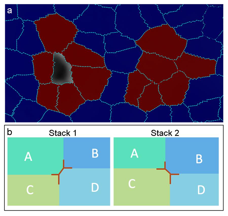
Figure 9. Examples of lineage tracing errors. (a) Two major types of errors. Left: Most likely due to incorrect parental labeling or in correct segmentation, e.g., Stack 1 is over-segmented, but only one of the cells can be mapped to Stack 2. Right: Most likely due to incorrect cell junctions. (b) An example of why junction error can occur. In Stack 1, Cell A and D were physically connected to each other, but C and B were not, while in Stack 2, C and B were physically connected to each other.
Data analysis
After all the errors are corrected, reload Meshes 1 and 2 to Stacks 1 and 2, respectively. Make sure Stack 2 is active and the Parents box is checked. Under the Process tab, run Mesh → Lineage Tracking → Load parents, and load the latest version of the parental tracing file.
For all the heat maps, the scale of the values can be changed in Process → Mesh → Heat Map → Heat Map Range; the styles can be changed by clicking the Colors Editor
 next to the view option of Cells in the Surface panel; and screenshots can be taken by clicking the Save screenshot
  on the main toolbar. All the original images from Min et al. (2022) were saved as .PNG in 2700 px (width) × 2500 px (height).
Heat maps of cell area expansion and cell proliferation
To create a heat map for cell area expansion, under the Process tab, run Process → Mesh → Heat Map → Heat Map Classic. Select “Area” for the heat map type and “Geometry” for the visualization. Differences in various change map options can be found on the MorphoGraphX manual. Also select the “Change map” checkbox. This tells MorphoGraphX to make a heat map comparing Stack1 and Stack2. The heat map can be visualized on either the first (typically, Stack 1) or second (Stack 2) time points. For the growth sample here, select “Increasing” if Stack 1 (i.e., time-point 1) is active or “Decreasing” if Stack 2 (i.e., time-point 2) is active.
To create a map of cell proliferation, make sure Stack 2 is active, and run Process → Mesh → Lineage Tracking→ Heat Map Proliferation.
To create images such as Figure 3 in Min et al. (2022), in which divided cells are highlighted on a cell area extension heat map, first run cell area expansion heat map on Stack 2. Check “Report to spreadsheet” so that the values of cell area expansion for each cell can be saved. Give the spreadsheet an informative name, such as “r8-A1-tp1_tp2-growth-allcells.csv”. Then create a map of cell proliferation by running Process → Mesh → Lineage Tracking→ Heat Map Proliferation. Subsequently, run Process → Mesh → Heat Map → Heat Map Select, and change the range values: Lower Threshold to 2, and Upper Threshold to 3 or higher. This step will select all the cells that have experienced cell division. Then, go to Process → Mesh → Heat Map → Heat Map Load, load “r8-A1-tp1_tp2-growth-allcells.csv” as the Heat Map file, and make sure the Column to load is set as “Value”.
The aesthetics of the growth heat map and cell outlines can be changed in the Main tab. To change the cell outlines, go to Main → Stack 1 → the Colors Editor
by the Mesh panel. To change the heat map styles, go to Main → Stack 2 (if heat map is displayed on Stack 2) → the Colors Editor by the Cells in the Surface panel. Sometimes, the heatmap color scale appears to be incorrect on the screen. This is most likely to happen when both Stack 1 and Stack 2 are displaying heat maps, and the color scale of Stack 1 will cover the color scale of Stack 2. This can be simply solved by unclicking the Surface panel under Stack 1.
Heat maps of principle direction of growth and anisotropy
Make sure the parental file has been loaded to Stack 2, and then switch to Stack 1 to designate it as the active stack. Under the Process tab, run Mesh → Cell Axis → PDG → Check Correspondence, No error should show up since the meshes have been corrected. Make sure the active Stack is the stack that you want to display the heat map on, so if you want to display heat map on time-point 2, make Stack 2 as the active stack. Then run Mesh → Cell Axis → PDG → Compute Growth Directions. The PDG values can also be saved by running Mesh → Cell Axis → Cell Axis Save. Detailed explanations of the PDG parameters can be found in the MorphGraphX manual.
To change the display of the PDG map, go to Mesh → Cell Axis → PDG → Display Growth Directions. The PDG heat maps in Min et al. (2022) were displayed as Anisotropy, which is the ratio between StretchMax and StretchMin. A ratio of 1 means no deformation, 2 means an elongation of 100%, and 0.8 a shrinkage of 20%. The color and size of the PDG vectors can also be modified. By default, vectors corresponding to expansion (stretch ratio > 1) are displayed in white, while red is used to draw the direction of shrinkage (stretch ratio < 1). The “Threshold” parameter is used to display PDGs axis only in cells for which the anisotropy is above a given value. Since we save each image at a relatively high resolution (2700 × 2500), we found that a Line Width of at least 10 px is needed for good visualization on the final screenshot.
Perspectives
In this study, we presented the first quantitative live-imaging protocol of floral buds of A. coerulea, which offers considerable potential for application to other non-traditional plant systems. This step-by-step guide offers an important source of basic information for non-model researchers who can take the core of the protocol and adapt it according to the needs of their system. Some aspects of any live imaging project will be specific to the species and/or tissue; therefore, dissection methods, sterilization time, media recipes, and staining times are all likely to be elements that will require optimization. Additionally, there is still room for improvement to obtain higher quality quantitative data. First, our samples were stained with propidium iodide (PI), which generally gave good signal in most of the tissue, but cells in the organ boundary regions were often under-stained. Repetitive long-term staining with PI is known to become toxic to tissues and thus slow growth (Grandjean et al., 2004; Bureau et al., 2018), which was also the primary factor that restricted the length of the analyzed developmental window. Further development of transgenic markers for the plasma membrane would help to solve these issues. Second, our analysis was limited to surface reconstruction of the cells, although the behavior of cells under the epidermal layer is an indispensable part of fully understanding meristem morphogenesis. Third, due to the imaging mechanisms of the available confocal microscope, cell walls perpendicular to the focal axis of the microscope were often not detected. Combined with the fact that cells at the organ boundary were often poorly stained, we were often unable to segment and analyze cells in many boundary regions on the abaxial side of some primordia. Except for the issue with PI staining, all of the other limitations described here are, in fact, challenges faced by similar studies in the established model systems (Rambaud-Lavigne and Hay, 2020; Prunet and Duncan, 2020). Fortunately, rapid development in microscopes that allow long-term, deep-tissue, minimally invasive scanning, as well as software developments that can segment and reconstruct multiple cell layers in 3D from the imaging data, are in progress. A comprehensive understanding of "the genetics of geometry" (Coen et al., 2004) of morphogenesis in a diverse set of plant systems is hopefully underway.
Recipes
Culture medium
To make up 1 L of the culture medium, dissolve 2.375 g of Linsmaier & Skoog medium (Fisher Scientific; final strength: 0.5×) and 30 g of sucrose (final concentration: 3%) in 1 L of ddH2O. The Linsmaier & Skoog medium should provide buffering capacity such that the pH of the solution should be approximately 5.8. If the pH is too high, adjust it with 1N NaOH solution. Then, add 8 g of agar (final concentration: 0.8%), and autoclave.
Once the autoclaved medium has cooled to a degree that is not too hot to be touched by a bare hand, add 10-6 M kinetin (Sigma) and 10-7 M gibberellic acid (GA3, Sigma). Do not reheat the culture media once hormones have been added. Mix well and pour the plates in a fume hood, to avoid contamination. 10-6 M kinetin and 10-7 M GA3 can be diluted as follows:
10-6 M kinetin
Make 10-1 M stock solution: dissolve 21.52 mg kinetin in 1 mL of 1 N NaOH in an Eppendorf tube. Seal the tube tightly with parafilm. This stock solution can be stored at 4°C for a few months.
Add 1 µL of the stock solution in 100 µL of ddH2O, to reach the concentration of 10-3 M.
Add 1 µL of 10-3 M solution in every 1 mL of culture medium, to reach a concentration of 10-6 M.
10-7 M GA3:
Make 10-1 M stock solution: dissolve 34.64 mg GA3 in 1 mL of EtOH in a 1.6 mL Eppendorf tube. Seal the tube tightly with parafilm. This stock solution can be stored at 4°C for a few months.
Add 1 µL of the stock solution in 1 mL of ddH2O to reach the concentration of 10-4 M.
Add 1 µL of 10-4 M solution in every 1 mL of culture medium, to reach a concentration of 10-7 M.
Acknowledgments
This study was funded by the Emerging Models Grant from the Society of Developmental Biology.
Competing interests
The authors declare no conflicts of interest.
References
- Bureau, C., Lanau, N., Ingouff, M., Hassan, B., Meunier, A. C., Divol, F., Sevilla, R., Mieulet, D., Dievart, A. and Perin, C. (2018). A protocol combining multiphoton microscopy and propidium iodide for deep 3D root meristem imaging in rice: application for the screening and identification of tissue-specific enhancer trap lines. Plant Methods 14: 96.
- Caggiano, M. P., Yu, X., Ohno, C., Sappl, P. and Heisler, M. G. (2021). Live Imaging of Arabidopsis Leaf and Vegetative Meristem Development. Methods Mol Biol 2200: 295-302.
- Coen, E., Rolland-Lagan, A. G., Matthews, M., Bangham, J. A. and Prusinkiewicz, P. (2004). The genetics of geometry.Proc Natl Acad Sci U S A 101(14): 4728-4735.
- Geng, Y. and Zhou, Y. (2019). Confocal Live Imaging of Shoot Apical Meristems from Different Plant Species. J Vis Exp(145): e59369.
- Grandjean, O., Vernoux, T., Laufs, P., Belcram, K., Mizukami, Y. and Traas, J. (2004). In Vivo Analysis of Cell Division, Cell Growth, and Differentiation at the Shoot Apical Meristem in Arabidopsis. The Plant Cell 16(1): 74-87.
- Min, Y., Conway, S. J. and Kramer, E. M. (2022) Quantitative live-imaging of floral organ initiation and floral meristem termination in Aquilegia. Development 149 (4): dev200256
- Prunet, N. and Duncan, K. (2020). Imaging flowers: a guide to current microscopy and tomography techniques to study flower development. J Exp Bot 71(10): 2898-2909.
- Prunet, N., Jack, T. P. and Meyerowitz, E. M. (2016). Live confocal imaging of Arabidopsis flower buds. Dev Biol 419(1): 114-120.
- Rambaud-Lavigne, L. and Hay, A. (2020). Floral organ development goes live. J Exp Bot 71(9): 2472-2478.
- de Reuille, P. B., Robinson, S. and Smith, R. S. (2014). Quantifying cell shape and gene expression in the shoot apical meristem using MorphoGraphX. Methods Mol Biol 1080: 121-134.
- Steeves, T. A. and Sussex, I. M. (1989). Patterns in plant development. Cambridge University Press.
- Strauss, S., Sapala, A., Kierzkowski, D. and Smith, R. S. (2019). Quantifying Plant Growth and Cell Proliferation with MorphoGraphX. Methods Mol Biol 1992: 269-290.
- Shi, B., Wang, H. and Jiao, Y. (2020). Live Imaging of Arabidopsis Axillary Meristems. Methods Mol Biol 2094: 59-65.
- Silveira, S. R., Le Gloanec, C., Gomez-Felipe, A., Routier-Kierzkowska, A. L. and Kierzkowski, D. (2022). Live-imaging provides an atlas of cellular growth dynamics in the stamen. Plant Physiol 188(2): 769-781.
Article Information
Copyright
© 2022 The Authors; exclusive licensee Bio-protocol LLC.
How to cite
Min, Y., Conway, S. J. and Kramer, E. M. (2022). Quantitative Live Confocal Imaging in Aquilegia Floral Meristems. Bio-protocol 12(12): e4449. DOI: 10.21769/BioProtoc.4449.
Category
Cell Biology > Cell imaging > Confocal microscopy
Developmental Biology > Morphogenesis > Organogenesis
Plant Science > Plant developmental biology > Morphogenesis
Do you have any questions about this protocol?
Post your question to gather feedback from the community. We will also invite the authors of this article to respond.