Materials and Reagents

Animals
1. GCaMP6f^flox mice (Jackson Laboratory, catalog number: 028865)
2. Mist1^CreERT2 (Jackson Laboratory, catalog number: 029228)
Materials
1. 1 mL syringe (BD Biosciences, catalog number: 309659)
2. 27 G needle (BD Biosciences, catalog number: 305109)
3. Feeding tubes (Instech, catalog number: FTP-22-25)
4. Mouse restrainer/stage (Custom-made by 3D printer, Figure 1A)
5. Gland holder (Custom-made by 3D printer, Figure 1A)
6. Tungsten wire, 0.125 mm (WPI, catalog number: TGW0515)
7. Cover glass, 18 mm diameter (Fisherbrand, catalog number: 12-545-100)
8. Hand warmer (Kobayashi Consumer Products, Hothands)
9. Cotton sponge (Covidien, Curity 9022)
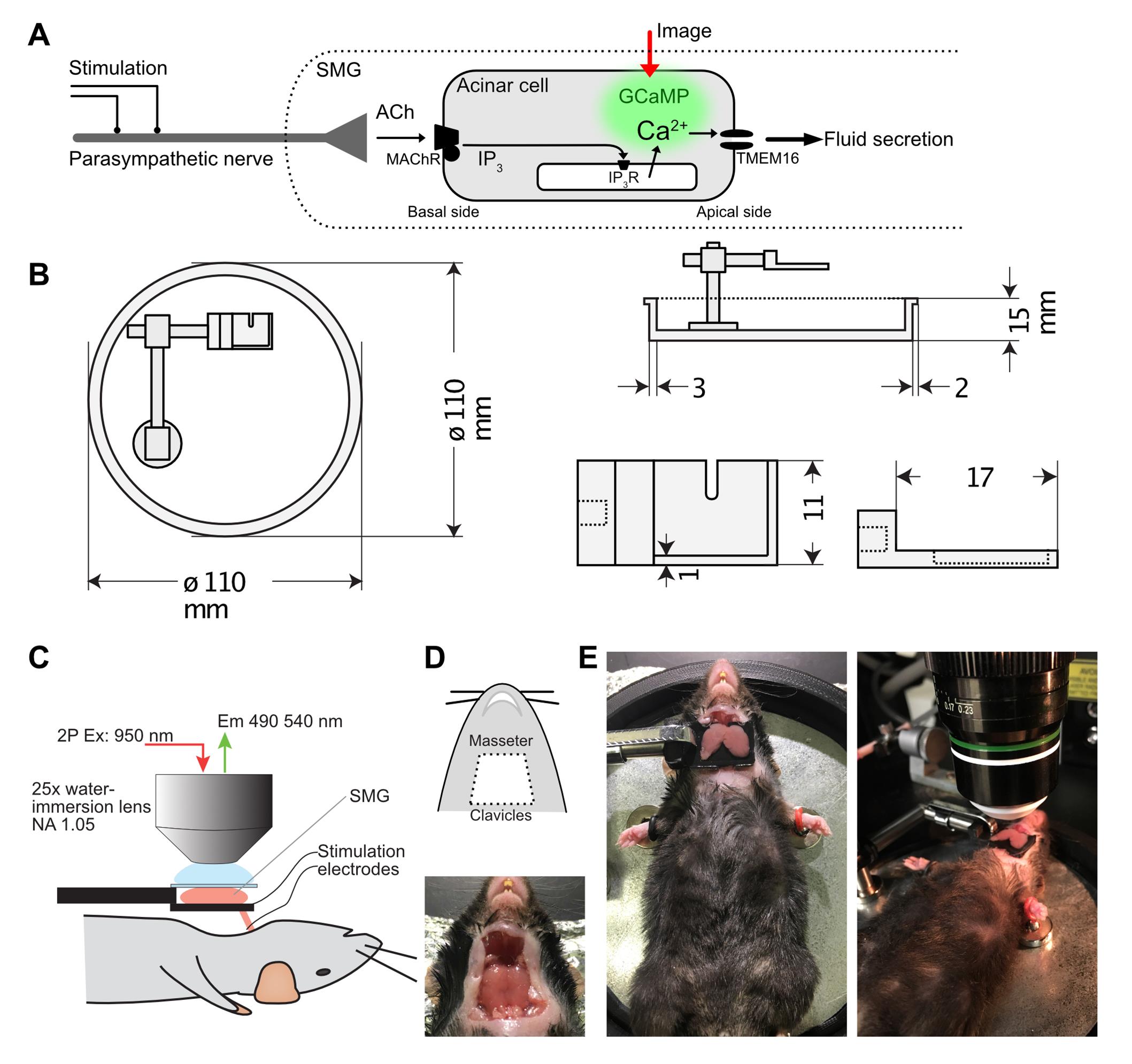
Figure 1. Design of in vivo salivary gland imaging setup. A. A cartoon depicting calcium signaling in acinar cells of the salivary gland. Neuronal input and acinar cell architecture are preserved only in vivo. Nerve input can be electrically initiated, and acinar calcium signaling optically observed in real time with the genetically-encoded calcium probe GCaMP6F. B. Design diagrams of the animal restrainer stage and gland holder. C. A diagram of the 2-photon imaging arrangement. D. Position of skin incision and a photograph of the exposed submandibular gland (SMG). E. Photographs of the SMG placed on a holder, with a cover glass flattening its surface, and an objective lens situated on top of the gland.
Reagents
1. Tamoxifen (Sigma-Aldrich, catalog number: T5648)
2. Corn Oil (Sigma-Aldrich, catalog number: C8267)
3. Ketamine (Hospira, Ketamine HCl, NDC 0409-2051-15)
4. Xylazine (Akorn Animal Health, AnaSed, NDC 59399-110-20)
5. Hank’s salt solution with calcium and magnesium, no phenol red (Gibco, catalog number: 14025-092)
6. Hair remover (Church & Dwight, Nair)
7. Ethanol, 200 proof (Koptec, V1001)
8. Petroleum jelly (Unilever, Vaseline)
9. Tamoxifen stock solution (see Recipes)
10. Salivary gland holder (see Recipes)

Equipment

Stereo microscope (LW Scientific, Z4)
Surgical scissors (Fine Science Tools, catalog number: 91460-11)
Forceps (Fine Science Tools, catalog number: 11252-40)
Two-photon laser-scanning microscope (Olympus, FVMPE-RS)
25× water-immersion objective lens (Olympus, XLPlan NA 1.05 W MP)
Ti:Sapphire laser (Spectra-Physics, Insight X3)
Objective lens heater (OKOLab COL2532)
Stimulus Isolator (A.M.P.I., Iso-flex)
Pulse generator (Digitimer Ltd, DG2A)

Software

FV31s-SW (Olympus, FV31s-SW)
FIJI/ImageJ (NIH, https://imagej.net/software/fiji/)
Prism (GraphPad)

Procedure

Generation of mice expressing GCaMP6f in exocrine acinar cells
1. To generate Mist1^+/–;GCaMP6f^+/– transgenic mice, cross 2–7 months old female homozygous GCaMP6f^flox mice (Jackson Laboratory; 028865) with 2–9 months old male heterozygous Mist1^CreERT2 (Jackson Laboratory; 029228). Genotyping was carried out according to protocols supplied by the Jackson Laboratory (Genotyping protocols 27076 and 20626, respectively).
2. To induce GCaMP expression in acinar cells, treat Mist1^+/–;GCaMP6f^+/– mice at least 6 weeks old with tamoxifen. Prepare 60 mg/mL tamoxifen in corn oil, and administer 0.25 mg/g body weight by oral gavage once a day for three consecutive days, using a plastic feeding tube attached to a 1 mL syringe. Imaging is carried out 1–4 weeks after the last tamoxifen administration.
Animal preparation
1. Anesthetize the animal with Ketamine [80 mg/kg body weight, intraperitonially (i.p.)] and Xylazine (10 mg/kg body weight, i.p.). Place the animal on a custom-made mouse-restrainer with the ventral side up (Figure 1C–E ). Place a heat pad (HotHands, Kobayashi) under the restrainer and wrap the animal’s body with a cotton sheet, to prevent hypothermia. Perform a toe-pinch intermittently, at least every 10–20 min, to evaluate the depth of anesthesia. Additional anesthetic of 20–40 mg/kg ketamine, is given when necessary.
2. To remove hair at the surgical region, apply hair remover cream to the animal’s neck, then wipe with 70% ethanol. With a pair of scissors, make an incision at the neck just anterior to the clavicles, through the end of the masseter muscle (Figure 1D). Lift the incised skin to expose the submandibular/sublingual glands. Carefully tease away connective tissues surrounding the gland using two pairs of forceps, until the gland is detached from the body, except by a bundle composed of blood vessels, nerve, and the secretory duct, at the anterior side of the gland (Figures 1C–E ).
3. Lift the gland and insert a pair of tungsten wires to the bundle, one at the base near the body, and the other at where the bundle is connected to the gland. Connect the other ends of the wires to the stimulator.
4. Place the gland on a 11 × 17 mm custom build small holder situated directly above the neck, so that the position of the gland is not influenced by movement as a result of breathing (Figure 1C, 1E). Apply Hanks salt solution in the holder, apply petroleum jelly or silicone gel at the edge of the holder, then place a cover glass onto the gland, so that the surface of the gland is flattened, but the gland is not overtly squeezed by pressure.
In vivo imaging
1. Attach an objective heater to the 25× water immersion lens prior to the imaging session, to equilibrate the lens temperature to 37°C. Tune the excitation laser connected to an upright microscope at 950 nm. Set the emission filter at 495–540 nm.
2. Place the animal on the microscope stage. Apply Hank’s solution between the objective lens and the cover glass holding the gland. Turn on a gooseneck light source and adjust the focus in bright field view through eyepieces. Find a flat clean region of the submandibular gland for imaging. Connect the stimulator to the pulse generator. Turn off the light source and keep the microscope stage dark, by covering the microscope with a black curtain and keeping the room dark. Set the resonance scanner of the FV31s-SW laser-scanning system to 30 frames per second, and collect an average of 3 frames as a single frame, to achieve a 10 fps image collection rate. The image resolution is 512 × 512 pixels, and the magnification is adjusted by zooming with scanner control, typically from 2× to 4× zoom.
3. Adjust the laser power so that the baseline fluorescence is faintly visible, about 20% of saturation (Figure 2A). PMT settings are fixed at 600 V, 1× gain, and 3% black level. Find the surface of that gland by moving focus, and set the registered depth as 0 µm. We typically image at depths between 10 and 55 µm from the surface of the gland. Adjust the laser power as depth changes.
  
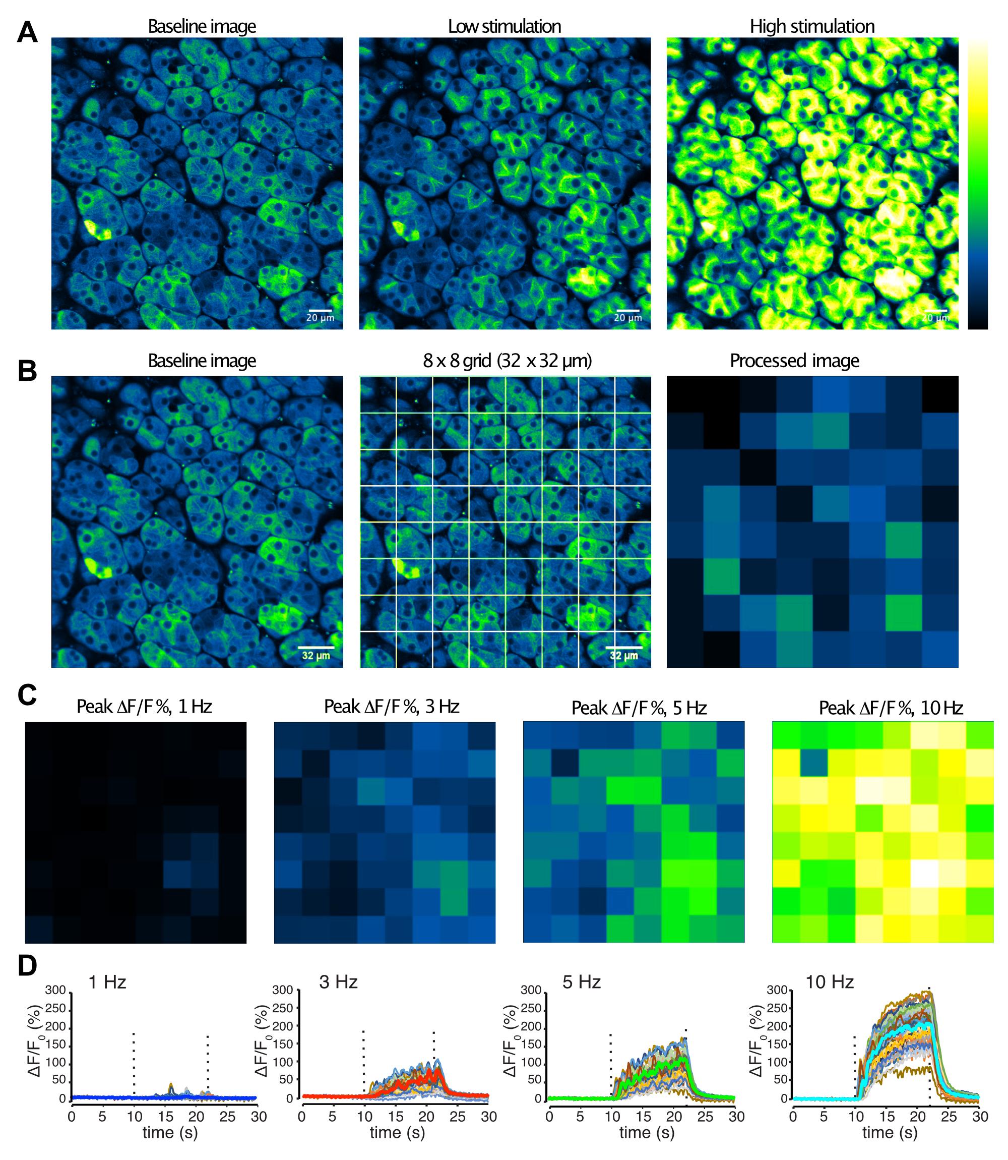
  Figure 2. Image analyses of in vivo salivary gland imaging. A. Images of acinar cells in submandibular gland before, and during low (3 Hz), or high (10 Hz) stimulations. B. Post-processing for spatio-temporal patterns of Ca²⁺ by nerve input. The image was subdivided into 8 × 8 grids, and average fluorescence intensity was obtained for each grid. C–D. Grid-analyses of an imaging field responding to 1–10 Hz stimulation. Grid images showing peak intensities (C) and time-course plots. Stimulation at the indicated frequency was applied between 10–22 s (D).
4. A test time-course set of images is taken for 30 s without external stimulation. Acinar cell fluorescence should be stable without spontaneous flickering, and the imaging field should not drift in XY or Z directions.
5. Start the image collection set from 30 s to 5 min. During the image collection, deliver a train of electrical stimulation using a stimulus isolator set at 5 mA for 200 µs, controlled by a pulse generator set to 1–10 Hz, for 12 s up to 5 min (Figure 2A). After a series of images are captured, allow 1–5 min of resting time before the next image capture, to let the tissue fully recover from the stimulation applied.
6. For line scan imaging, find an acinar cell cluster that is orientated in the image plane, such that apical and basal sides of the acinar cell are clearly identified, and the imaging plane depth crosses near the center of the cell (Figure 3A). After the capture of a single image of a chosen field, a line is drawn in the image from the apical end, passing through the nucleus, to the basal aspect of an acinar cell. The scanning speed of the line varies according to the length of the line, and is typically 1–1.6 ms per line (Figure 3B).
  
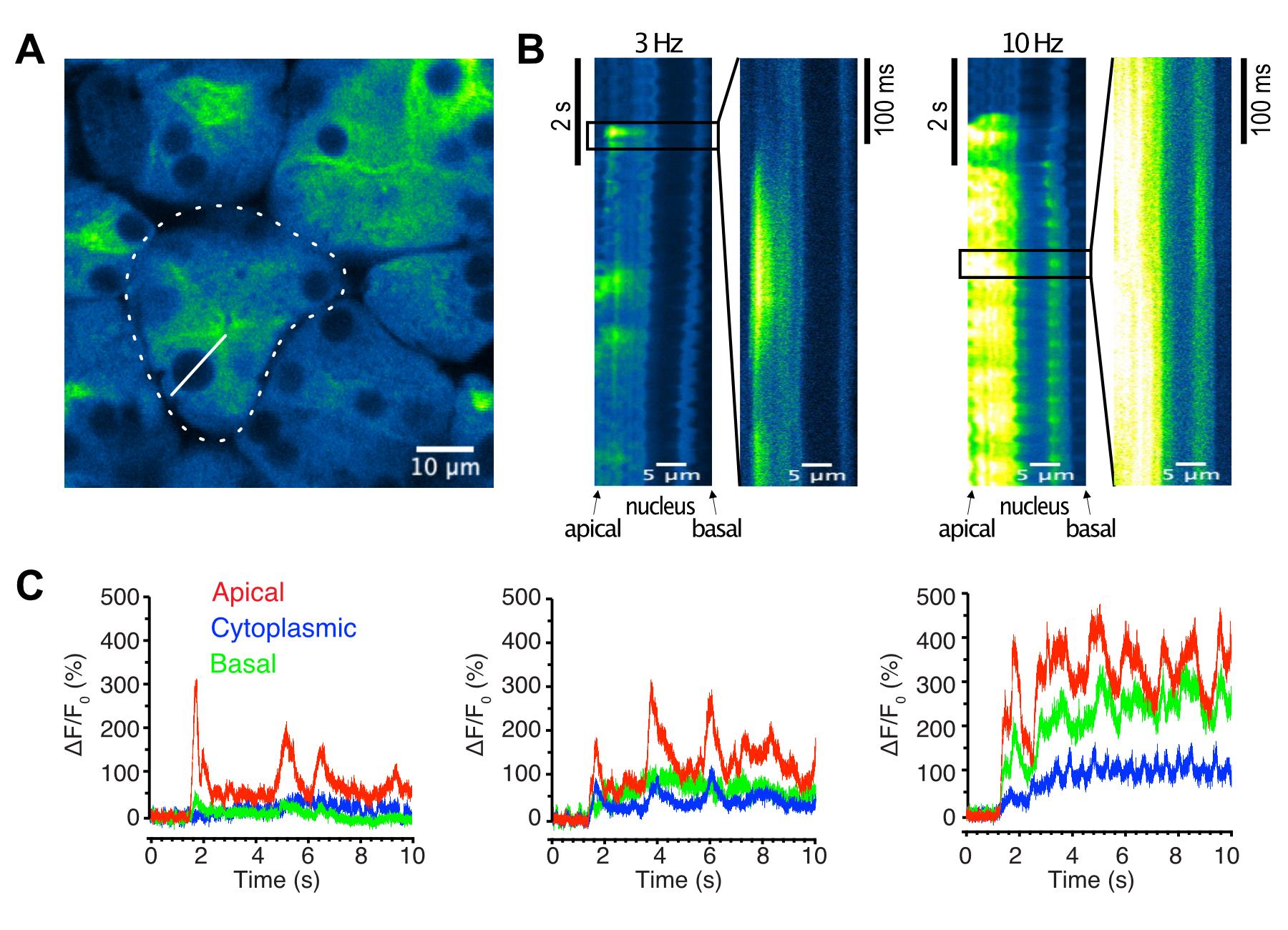
  Figure 3. Image analyses of line-scan salivary gland imaging. A. An image of a lobule showing radial arrangement of acinar cells, with the apical side at the center and the basal side at the circumference (dotted line). A line was defined in a cell from the apical end through the nucleus until the basal end (solid line). B. Line scan images across an acinar cell during 3 or 10 Hz stimulation, showing localization of Ca²⁺ at the apical side of the cell without intracellular Ca²⁺ spread toward the basal side. C. Time-course plots from regions of interest (ROI’s) representing the apical (red), cytoplasmic (blue), and basal (green) regions, responding to 3 Hz (left panel), 5 Hz (middle panel), and 10 Hz (right panel) stimulations.
7. Continue to perform a toe-pinch intermittently, at every 10–20 min, to evaluate the depth of anesthesia. Additional anesthetics of 20–40 mg/kg ketamine is given when necessary. Otherwise, administer 0.1 mL of saline solution every 30 min, to prevent dehydration. After the imaging, the animals are euthanized under anesthesia, according to a procedure approved by the University Committee on Animal Resources.

Data analysis

Open the acquired image in FIJI/ImageJ. Stimulation may cause mild drifting of the imaging field in the XY direction, so that the image series may have to be realigned to keep the cells in stationary positions throughout the time-course. For this, apply a descriptor-based series registration plugin (by Stephan Preibisch, included in the FIJI package) using the nucleus, appearing as blank fixed-size round spots, as references for positioning.
For whole field average Ca²⁺ changes over time, select the whole image using the ROI Manager, and measure mean gray values for each frame with the Multi Measure function. An average of gray values in frames before stimulation serves as the baseline value (F₀), and %∆F/F₀ [(F– F₀)/ F₀ × 100] is then calculated for all the frames in a series. The standard deviation (SD) of the 100 baseline frames from grids in each image series provides an estimate of the noise level. A change >4 SD from the F₀ value is considered as an evoked Ca²⁺ signal.
For analyses of heterogeneity of Ca²⁺ responses in acinar cells stimulated in an imaging field, rather than manually identify each cell, whose sizes and shapes vary greatly, and whose cell boundaries are not always apparent, we divide the field into 8 x 8 grids. This yields 64 ROIs, which correspond to dimension of 32 × 32 µm² for images taken with a 25× objective, 512 × 512 pixel size, with zoom 2× (Figure 2B). The average intensity of each ROI grid is generated for each frame. The average of the first 100 frames prior to stimulation serves as baseline fluorescence (F₀), and %∆F/F₀ [(F– F₀)/F₀ × 100] is calculated, using the Image calculator function, so that the converted 32-bit image series represents [Ca²⁺] changes over time expressed as %∆F/F₀ in 8 × 8 alley of grids in the XY dimension (Figures 2B–D ). Of note, we confirmed the validity of this analysis scheme by comparing information obtained from 8 × 8 grids to 16 × 16 grids, and randomly and manually selected individual acinar cells. Each scheme produced essentially equivalent data.
The percentage of acinar calls responding to a particular stimulation frequency is evaluated by counting the numbers of grids that showed at least one response above the noise level during the stimulation duration. To calculate the latency prior to a measurable response, the time to the first observed Ca²⁺ signal that meets the criteria as responding after the initiation of the stimulation are recorded. Non-responding grids are excluded from the latency analysis. Peak Ca²⁺ amplitude is obtained by extracting maximum %∆F/F₀ values during the stimulation duration from each grid.
For XT-line scan images, we separate the line into three zones, to represent the basal, cytosolic, and apical regions. The line contains the nucleus, which appears as a dark band near the basal side, and this band separates the basal region from the cytosolic and apical regions (Figure 3A, 3B). Each region is defined as a 3 µm wide line within the image, and fluorescent intensity before stimulation for each region serves as the baseline intensity (F₀ = 0%) (Figure 3C).
All statistical analyses are performed with paired t test, one-way ANOVA, and linear regression, using Prism (GraphPad).

Recipes

Tamoxifen stock solution
Tamoxifen powder: 600 mg
Corn oil: 10 mL
Heat to 70°C until dissolved.
Salivary gland holder
Thorlabs, ER1 Assembly rods, ×3
Thorlabs, ER90B angle clamps, ×2
Permanent Magnet, Round, ½” diameter
Holder tray, made with 3D printer

Acknowledgments

We thank Dr. Catherine Ovitt, University of Rochester, for providing Mist1^CreERT2 mice, Multiphoton and Analytical Imaging Center for providing Olympus FV31s-SW multiphoton system, and our laboratory members for valuable input and help. This work was supported by NIH grants RO1DE019245 and RO1DE014756. Research using this protocol was published in Takano et al. (2021; doi: 10.7554/eLife.66170).

Competing interests

The authors declare no conflicts of interest.

References

Ambudkar, I. S. (2011). Dissection of calcium signaling events in exocrine secretion.Neurochem Res 36(7): 1212-1221.
Ambudkar, I. S. (2016). Calcium signalling in salivary gland physiology and dysfunction. J Physiol 594(11): 2813-2824.
Arreola, J., Melvin, J. E. and Begenisich, T. (1996a). Activation of calcium-dependent chloride channels in rat parotid acinar cells.J Gen Physiol 108(1): 35-47.
Arreola, J., Park, K., Melvin, J. E. and Begenisich, T. (1996b). Three distinct chloride channels control anion movements in rat parotid acinar cells.J Physiol 490 ( Pt 2): 351-362.
Begenisich, T. and Melvin, J. E. (1998). Regulation of chloride channels in secretory epithelia. J Membr Biol 163(2): 77-85.
Futatsugi, A., Nakamura, T., Yamada, M. K., Ebisui, E., Nakamura, K., Uchida, K., Kitaguchi, T., Takahashi-Iwanaga, H., Noda, T., Aruga, J. and Mikoshiba, K. (2005). IP3 receptor types 2 and 3 mediate exocrine secretion underlying energy metabolism. Science 309(5744): 2232-2234.
Gallacher, D. V. and Petersen, O. H. (1983). Stimulus-secretion coupling in mammalian salivary glands. Int Rev Physiol 28: 1-52.
Lee, M. G., Xu, X., Zeng, W., Diaz, J., Wojcikiewicz, R. J., Kuo, T. H., Wuytack, F., Racymaekers, L. and Muallem, S. (1997). Polarized expression of Ca²⁺ channels in pancreatic and salivary gland cells. Correlation with initiation and propagation of [Ca²⁺]_i waves. J Biol Chem 272(25): 15765-15770.
Maruyama, Y., Gallacher, D. V. and Petersen, O. H. (1983). Voltage and Ca²⁺-activated K⁺ channel in baso-lateral acinar cell membranes of mammalian salivary glands. Nature 302(5911): 827-829.
Matsui, M., Motomura, D., Karasawa, H., Fujikawa, T., Jiang, J., Komiya, Y., Takahashi, S. and Taketo, M. M. (2000). Multiple functional defects in peripheral autonomic organs in mice lacking muscarinic acetylcholine receptor gene for the M3 subtype.Proc Natl Acad Sci U S A 97(17): 9579-9584.
Melvin, J. E. (1991). Saliva and dental diseases. Curr Opin Dent 1(6): 795-801.
Nakamoto, T., Romanenko, V. G., Takahashi, A., Begenisich, T. and Melvin, J. E. (2008). Apical maxi-K (KCa1.1) channels mediate K⁺ secretion by the mouse submandibular exocrine gland. Am J Physiol Cell Physiol 294(3): C810-819.
Nakamoto, T., Srivastava, A., Romanenko, V. G., Ovitt, C. E., Perez-Cornejo, P., Arreola, J., Begenisich, T. and Melvin, J. E. (2007). Functional and molecular characterization of the fluid secretion mechanism in human parotid acinar cells. Am J Physiol Regul Integr Comp Physiol 292(6): R2380-2390.
Pages, N., Vera-Siguenza, E., Rugis, J., Kirk, V., Yule, D. I. and Sneyd, J. (2019). A Model of [Formula: see text] Dynamics in an Accurate Reconstruction of Parotid Acinar Cells. Bull Math Biol 81(5): 1394-1426.
Pedersen, A. M., Bardow, A., Jensen, S. B. and Nauntofte, B. (2002). Saliva and gastrointestinal functions of taste, mastication, swallowing and digestion. Oral Dis 8(3): 117-129.
Putney, J. W., Jr. (1982). Cellular regulation. Science 216(4553): 1403-1404.
Romanenko, V. G., Catalan, M. A., Brown, D. A., Putzier, I., Hartzell, H. C., Marmorstein, A. D., Gonzalez-Begne, M., Rock, J. R., Harfe, B. D. and Melvin, J. E. (2010a). Tmem16A encodes the Ca²⁺-activated Cl^- channel in mouse submandibular salivary gland acinar cells. J Biol Chem 285(17): 12990-13001.
Romanenko, V. G., Nakamoto, T., Srivastava, A., Begenisich, T. and Melvin, J. E. (2007). Regulation of membrane potential and fluid secretion by Ca²⁺-activated K⁺ channels in mouse submandibular glands.J Physiol 581(Pt 2): 801-817.
Romanenko, V. G., Thompson, J. and Begenisich, T. (2010b). Ca²⁺-activated K channels in parotid acinar cells: The functional basis for the hyperpolarized activation of BK channels.Channels (Austin) 4(4): 278-288.
Takano, T., Wahl, A. M., Huang, K. T., Narita, T., Rugis, J., Sneyd, J. and Yule, D. I. (2021). Highly localized intracellular Ca²⁺ signals promote optimal salivary gland fluid secretion. Elife 10: e66170.
Weiss, S. J., McKinney, J. S. and Putney, J. W., Jr. (1982). Regulation of phosphatidate synthesis by secretagogues in parotid acinar cells. Biochem J 204(2): 587-592.
Won, J. H., Cottrell, W. J., Foster, T. H. and Yule, D. I. (2007). Ca²⁺ release dynamics in parotid and pancreatic exocrine acinar cells evoked by spatially limited flash photolysis. Am J Physiol Gastrointest Liver Physiol 293(6): G1166-1177.