- Protocols

- Articles and Issues
- For Authors
- About
- Become a Reviewer

Live-cell Imaging and Analysis of Germline Stem Cell Mitosis in Caenorhabditis elegans
Published: Vol 12, Iss 1, Jan 5, 2022 DOI: 10.21769/BioProtoc.4272 Views: 4741
Reviewed by: Gunar FabigDemosthenis ChronisAnonymous reviewer(s)
Original research article
The authors used this protocol in:
Apr 2021

Protocol Collections
Comprehensive collections of detailed, peer-reviewed protocols focusing on specific topics


Related protocols
Abstract
Model organisms offer the opportunity to decipher the dynamic and complex behavior of stem cells in their native environment; however, imaging stem cells in situ remains technically challenging. C. elegans germline stem cells (GSCs) are distinctly accessible for in situ live imaging but relatively few studies have taken advantage of this potential. Here we provide our protocol for mounting and live imaging dividing C. elegans GSCs, as well as analysis tools to facilitate the processing of large datasets. While the present protocol was optimized for imaging and analyzing mitotic GSCs, it can easily be adapted to visualize dividing cells or other subcellular processes in C. elegans at multiple developmental stages. Our image analysis pipeline can also be used to analyze mitosis in other cell types and model organisms.
Background
While permitting the visualization of various tissue-resident stem cells in several model systems, recent advances in intravital imaging often rely on invasive surgery or sophisticated and expensive imaging modalities ( Yoshida et al., 2007; Rompolas et al., 2012; Ritsma et al., 2014; Barbosa et al., 2015; Park et al., 2016; Martin et al., 2018; Nguyen and Currie, 2018). C. elegans GSCs are an established stem cell model that has yielded generalizable insights into many aspects of stem cell biology (Kimble and White, 1981; Baugh and Sternberg, 2006; Fielenbach and Antebi, 2008; Angelo and Van Gilst, 2009). In addition, C. elegans GSCs can be imaged in living animals using standard fluorescence microscopy techniques and without surgical manipulation. In particular, live imaging of GSC mitosis provides an opportunity to investigate the dynamics of cell division and how they are influenced by in vivo factors such as tissue organization, niche signaling, and organismal physiology. Here we describe a simple, fast, and reproducible method to immobilize C. elegans and to image and analyze GSC mitosis, while preserving animal viability, fertility, and seemingly normal GSC divisions.
Adult C. elegans hermaphrodites house two populations of GSCs located at the distal ends of the two tube-shaped gonad arms (Figure 1A). Like other germlines, the C. elegans gonad is organized as a syncytium. GSCs form a rough circumferential monolayer around a shared inner core of cytoplasm named the rachis (Hirsh et al., 1976) (Figure 1A and 1C). Each GSC is connected to the rachis by a stable actomyosin ring, which forms a cytoplasmic bridge (Maddox et al., 2005; Zhou et al., 2013; Amini et al., 2014; Priti et al., 2018). Like other stem cells, C. elegans GSCs are kept in a stem-like state by signaling from a somatic niche (the distal tip cell, Kimble and White, 1981; Figure 1A and 1E). Like several types of mammalian stem cells, the size of the C. elegans GSC pool is maintained according to a population model, wherein differentiation due to displacement from the niche is balanced by symmetrical divisions to maintain a relatively constant number of stem cells. according to a population model, wherein differentiation due to displacement from the niche is balanced by symmetrical divisions, thus maintaining a relatively constant number of stem cells (Morrison and Kimble, 2006; Joshi et al., 2010).
The majority of studies in C. elegans GSCs rely on dissected, fixed, and stained gonads, or single-timepoint imaging of gonads bearing fluorescently tagged proteins in living worms. Long-term imaging of GSCs has been accomplished using “catch and release” approaches that permit periodic visualization of GSCs over hours or days (Wong et al., 2013; Rosu and Cohen-Fix, 2017). Moreover, a recently developed microfluidics device may permit continuous observation on a similar time scale (Berger et al., 2018, Berger and Spiri, 2021). Fewer studies have reported live cell imaging of GSCs under conditions suitable for documenting dynamic subcellular events such as mitosis (Gerhold et al., 2015; Gordon et al., 2020; Zellag et al., 2021).
To achieve high temporal and spatial resolution during live imaging, animals must be immobilized and the overall impact of mounting on animal and GSC physiology must be considered. Typical mounting methods immobilize animals using a combination of paralytic drugs and physical compression (Sulston and Horvitz, 1977; Chai et al., 2012; Kim et al., 2013; Hwang et al., 2014; Luke et al., 2014; Burnett et al., 2018; Fabig et al., 2020a and 2020b; Gordon et al., 2020). We use an etched silicon wafer to pattern grooves on an agarose pad, which constrains the animals in a straight position (Figure 1B); this prevents the sinusoidal movements required for worm locomotion (Gray and Lissmann, 1964) and reduces the requirement for physical compression and anesthetics.
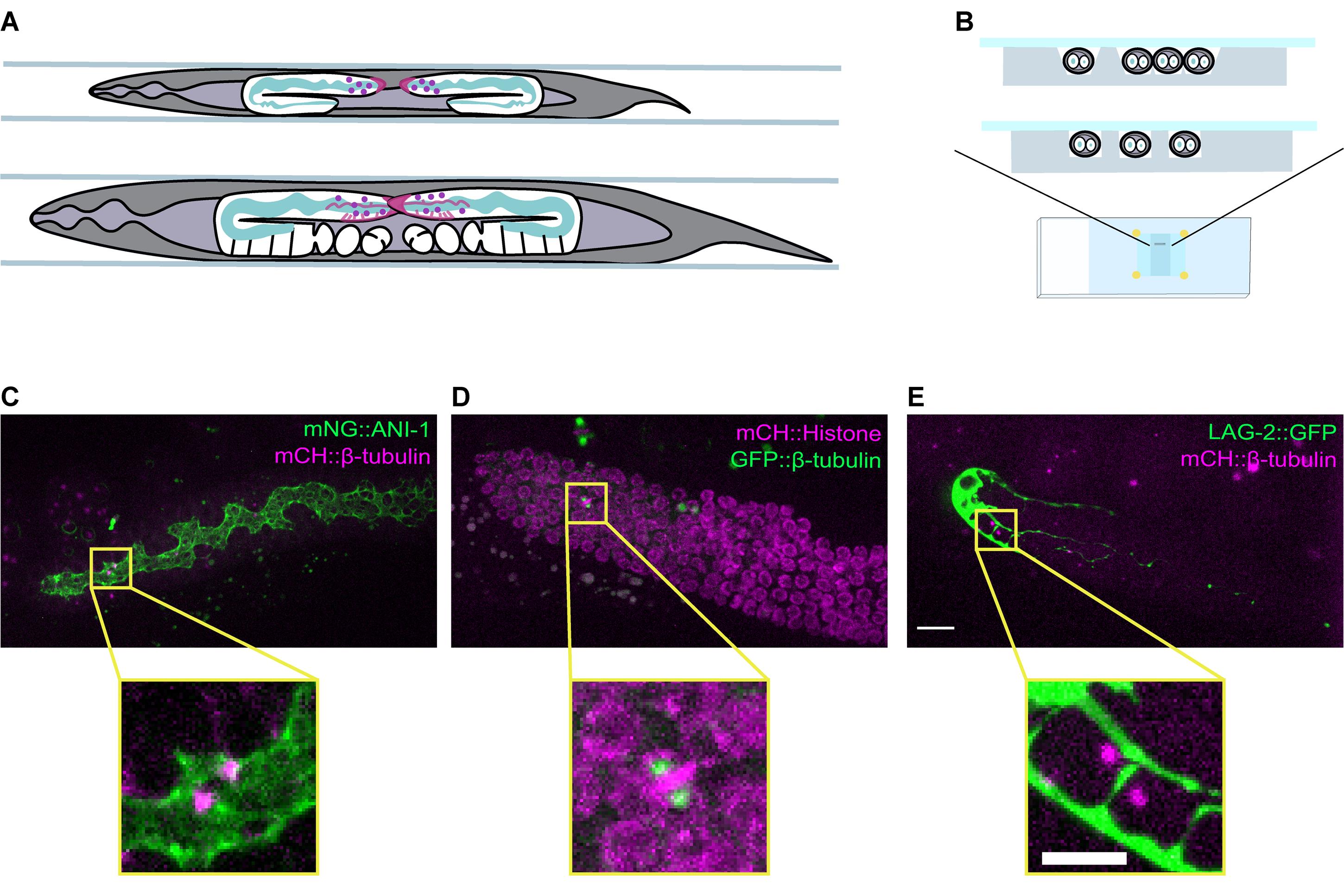
Figure 1. A mounting method allowing for live-imaging of dividing GSCs in intact C. elegans. A. Schematic showing a top view of a late L4 (top) and an adult (bottom) hermaphrodite worm mounted in grooves. The position and overall organization of the two gonad arms are shown in white, and key germline features are highlighted, such as the rachis (green), and the distal tip cell (DTC) or niche (magenta). The position of the GSCs is indicated by purple circles. B. Schematic showing a cross-sectional view of animals mounted in v-shaped (top) and square-shaped (bottom) grooves that match the width of the animals. (C-E) Maximum intensity projections of the distal gonad from adult animals expressing (C) mNG::ANI-1 (green) and mCH::β-tubulin (magenta; strain = UM679), D. GFP::β-tubulin (green) and mCH::Histone H2B (magenta; strain = JDU19), and (E) LAG-2::GFP (green) and mCH::β-tubulin (magenta; strain = UM211). A dividing GSC in each gonad is boxed in yellow and an enlarged image is shown below. Fluorescently labelled β-tubulin marks the mitotic spindle in all three strains, with mNG::ANI-1 marking the rachis, mCH::Histone H2B marking nuclei and LAG-2::GFP marking the DTC/niche. Scale bar = 10 µm (top, gonad view) and 5 µm (bottom, single cell view).
We have used this mounting method to provide the first characterization of GSC mitosis by live imaging (Gerhold et al., 2015). Recently, we investigated the technical factors that impact GSC mitosis during live imaging, which allowed us to define optimal mounting and imaging conditions, and to determine that animal starvation during mounting/imaging has the most deleterious effect on GSC mitosis (Zellag et al., 2021). Our data suggest that GSC mitosis can be imaged under near physiological conditions within an approximately 40 min window, which starts from the moment worms are removed from food. Although some GSCs enter mitosis after 40 min, we recommend caution when interpreting their behavior. In addition, under optimal conditions, the number of mitoses per germline and the duration of these mitoses in wild-type worms are relatively constant, and offer a reproducible baseline by which others may benchmark their results (see Videos 1 and 2 and Figure 4I-4K).
A parallel challenge that arises when using live imaging to study GSC mitosis is how to monitor mitotic progression. GSCs divide within the tube-shaped gonad and can divide in any orientation relative to the imaging plane, and at a range of depths relative to the gonad surface. Therefore, accurate monitoring of GSC mitosis requires a tracking method that accounts for the three-dimensional (3D) nature of their division. A good method will need to be sufficiently high-throughput to generate large data sets with minimal user time. In addition, fluorescently labelled proteins are often expressed at low levels in the germline (Merritt and Seydoux, 2010), which limits the availability of suitable markers.
We have shown that fluorescently tagged β-tubulin provides a robust marker for GSC mitotic centrosomes and that we can use centrosome-to-centrosome distance as a reliable readout for mitotic progression by tracking centrosome pairs in 3D (Gerhold et al., 2015; Zellag et al., 2021). In addition, tracking centrosome pairs can provide information on mitotic features, such as spindle dynamics and orientation (Zellag et al., 2021). To make this approach amenable to large-scale studies, we recently developed CentTracker, a largely automated image analysis pipeline that allows for fast extraction of mitotic parameters in any genetic background and in other cell types and organisms, provided that centrosomes are trackable (Zellag et al., 2021). Here, we describe the basic imaging processing steps required for using CentTracker. The relevant code and detailed instructions are freely available for download.
Materials and Reagents
60 mm Petri dish with cams (Sarstedt, catalog number: 82.1194.500)
1.5 mL microcentrifuge tube (Axygen, catalog number: MCT-150-C)
15 mL conical centrifuge tube (Fisher Scientific, catalog number: 14-959-53A)
Aspirator tube assembly for calibrated microcapillary pipettes (Sigma, catalog number: A5177-5EA)
50 µL glass micropipette (VWR, catalog number: 53432-783)
1.7 mL plastic transfer pipette (Fisher Scientific, catalog number: 13-711-41)
200 µL pipet tips (Diamed, catalog number: DIATEC520-6752)
1,250 µL pipet tips (Diamed, catalog number: DIATEC520-6501)
Single edge razorblade
Fine tipped forceps/tweezers
Lab tape (Fisher Scientific, catalog number: 15-901-10R)
18 × 18 mm #1.5 (0.16-0.19 mm) square cover glasses (VWR, catalog number: CA48366-205-1)
Microscope slides (Fisher Scientific, catalog number: 12-55-15)
Whatman 3 MM Chr blotting paper (VWR, catalog number: 21427-411), cut into ~3 cm strips
KIMTECK Kimwipes 11.2 × 21.3 cm
1-well glass depression slide (VWR, catalog number: 470235-728)
Silicon wafer micro-patterned by lithography, to give a series of parallel raised ridges with defined depth and width (Figure 2B-2C; see Note 1; hereafter “silicon mold”)
Worm pick [99.95% Platinum, 0.05% Iridium wire, 0.01 inches diameter (Tritech, catalog number: PT-9901), flattened like a spatula at one end, and mounted on a glass Pasteur pipette (Fisher Scientific, catalog number: 13-678-20A), or worm pick handle (Tritech, catalog number: TWPH1)]
Worm eyelash pick (see Note 2)
C. elegans strain(s) of preferred genotype bearing a fluorescent protein (FP) tagged centrosomal marker (if using CentTracker), with or without additional FP-tagged proteins (Figure 1C-1D; strains used in this protocol are listed in Table 1).
Note: We find that single-copy transgenes inserted by Mos1-mediated single copy insertion (MosSCI; Zeiser et al., 2011), or CRISPR-Cas9 with a single guide RNA (sgRNA) targeting a region near to established Mos1 insertion sites (Dickinson et al., 2013), and expressing FP-tagged proteins under the mex-5 promoter, and tbb-2 3’ UTR regulatory sequences produce the best results for germline-specific expression suitable for live-imaging.
Table 1. C. elegans strains used in this protocol.
Strain Genotype UM679 ltSi567[pOD1517/pSW222; Pmex-5::mCherry::tbb-2::tbb-2_3′UTR; cb-unc-119(+)] I; ani-1(mon7[mNeonGreen^3xFlag::ani-1]) III UM211 qls56[Plag2::GFP] V; wels21[Pja138(Ppie-1::mCherry::tubulin::pie-1_3’UTR)] ? JDU19 ijmSi7[pJD348/pSW077; mosI_5′mex-5_GFP::tbb-2; mCherry::his-11; cb-unc-119(+)] I; unc-119(ed3) III ARG16 ltSi567[pOD1517/pSW222; Pmex-5::mCherry::tbb-2::tbb-2_3′UTR; cb-unc-119(+)] I; ccm-3(mon9[ccm-3::mNeonGreen^3xFlag]) II E. coli strain OP50 (Brenner, 1974)
E. coli strain HT115 (Timmons and Fire, 1998)
Nematode Growth Medium (NGM) (Stiernagle, 2006; with the following modifications: 20 g agar and 3 g peptone per liter media)
Distilled water (dH2O)
10 M NaOH (Bioshop, catalog number: SHY700.1; powder dissolved in dH2O)
Commercial bleach (Bioshop, catalog number: SYP001.4; Sodium Hypochlorite, 12% Solution)
Vaseline® 100% pure petroleum jelly
Lanolin (Sigma, catalog number: L7387-250G)
Paraffin wax (Bernardin Parowax Canning Wax, 454g)
Tetramisole (Sigma, catalog number: L9756-5G)
Agarose powder (Sigma, catalog number: A9539-500G)
M9 buffer (see Recipes)
Bleaching solution (see Recipes)
Valap (see Recipes)
2% w/v Tetramisole solution (see Recipes)
3% w/v volume Agarose powder solution (see Recipes)
Equipment
Stereomicroscope with transmitted light stand (Leica, model: S6 E, Nikon, model: SMZ 745 or equivalent)
Note: We prefer stereomicroscopes with an external or LED light source, to avoid heating our worms during mounting.
Two heat blocks, one set to 95°C, and the other to 65°C (VWR, model: Standard Dry Block Heater or equivalent)
Benchtop microcentrifuge with rotor for 1.5-2 mL tubes (Eppendorf, model: 5415 D 24-tube with rotor F45-24-11, or equivalent)
Vortex mixer (Scientific Industries, model: Vortex-Genie 2, or equivalent)
Incubator set to 20°C (Sanyo, model: MIR-553, or equivalent)
Test tube rocker (Thermo Scientific, model: Vari-Mix M48725Q, or equivalent)
Single channel pipettes for 10-1,000 µL volumes (Gilson, models: Pipetman Classic P20, P200 and P1000, or equivalent)
Microwave
Spinning disc confocal microscope (Zeiss, model: Cell Observer, Quorum, model: WaveFX-X1, or equivalent) with excitation wavelengths and emission filters suitable for GFP and/or mNeonGreen and mCherry fluorescent proteins (e.g., 35-50 mW 488 nm or 491 nm, and 561 nm or 568 nm diode lasers, with ET525/50 and FF593/40 single band pass, or 466/523/600/677 quad band pass emission filters), and a high numerical aperture (NA) 63× oil objective (e.g., Leica, model: 63×/1.40-0.60 oil HCX PL APO, or Zeiss, model: 63× Plan-Apochromat DIC UV VIS-IR).
Note: If available, a high NA water immersion objective (e.g., Leica, model: HC PL APO 63×/1.20 W CORR CS2) may be preferable depending on the sample.
Spinning disk scanner (Yokogawa, model: CSU-X1)
Scientific CMOS camera (Zeiss, model: AxioCam 506 Mono, Photometrics, model: Prime BSI, or equivalent)
Software
Conda 4.9.0 or ulterior release (Anaconda, https://anaconda.org/anaconda/conda)
CentTracker Github repository: https://github.com/yifnzhao/CentTracker
Fiji 1.52v or ulterior release that includes TrackMate (Schindelin et al., 2012; Tinevez et al., 2017)
MATLAB 2020b or ulterior release (MathWorks, https://www.mathworks.com/products/matlab.html)
Procedure
Culture of C. elegans strains in preparation for GSC live imaging
Maintain C. elegans animals on nematode growth medium (NGM) inoculated with Escherichia coli strain OP50, according to standard protocols (Brenner, 1974).
Transfer worms regularly, to ensure a healthy and relatively synchronous population. We use a worm pick (Figure 2A) to transfer several small aggregates of ~L1 larvae (~50 animals in total) weekly (~every 2 generations) from plates maintained at 20°C, just as the bacterial lawn is becoming depleted. However, the optimal maintenance method will depend on the animals’ genotype and temperature at which they are grown (Stiernagle, 2006).
Table 1 lists the strains used in this study. To use CentTracker for analysis, animals must carry a centrosome marker suitable for fluorescence microscopy. We use β-tubulin tagged with either GFP or mCherry, which marks the mitotic spindle and is enriched at centrosomes. If a more specific centrosomal marker is needed, FP-tagged centriolar or pericentriolar components (e.g., SAS-4 or SPD-2; Magescas et al., 2019) may be more suitable.
Synchronization of larvae at the L1 stage
Three days in advance, set up plates by transferring 2-3 larger aggregates of recently starved L1 larvae from a stock plate to fresh NGM/OP50 plates, using a worm pick. This should ensure plates full of healthy, well-fed, and gravid adults when performing the synchronization procedure.
Note: Three days is appropriate timing if strains are maintained at 20°C; if strains require maintenance at another temperature, adjust this timing accordingly (Stiernagle, 2006).
Collect gravid adults by adding ~1 mL of sterile M9 to each plate. Once most animals are floating, use a P1000 pipetman to transfer the M9 and worms to a 1.5 mL microcentrifuge tube.
Spin tubes for 1 min in a benchtop microcentrifuge set to 4,000 × g, to collect animals into a loose pellet without damaging them.
Remove the M9 supernatant and discard.
Add 1 mL of bleaching solution (see Recipes).
Agitate the animals using a vortex mixer for approximately 6-7 min. This reaction should not be prolonged for more than 10 min. Check the condition of the animals using a stereomicroscope every ~1-2 min and stop the reaction as soon as the worms have started to lyse/break apart.
Immediately return tubes to the microcentrifuge and spin for 1 min at 4,000 × g.
Remove the bleaching solution from the worm carcasses and embryo pellet and add 1 mL of sterile M9.
Mix tubes on a vortex mixer for ~10 s and centrifuge for 1 min at 4,000 × g.
Remove the M9 and repeat this washing procedure two more times.
After the last spin, add 750 µL of sterile M9 to the worm pellet.
Incubate tubes at 15°C on a tube rocker for ~24 h to allow for L1 hatching. L1s hatching in the absence of food will remain in developmental diapause, thereby creating a synchronous population, which can be maintained at 15°C for 5-7 days.
On the day of use, determine the approximate concentration (L1s per µL) of surviving and arrested L1s in each tube, by counting the number of thrashing animals present in 10 µL of the M9 and starved L1 solution after inverting the tube several times to ensure an even distribution.
Use a P20 or P200 pipetman to transfer 10-15 synchronized L1s in M9 to a 35 mm NGM plate inoculated with HT115, using the number of L1s per µL from Step B13 to select the appropriate volume. To image late L4 larvae, incubate plates at 20°C for 40-48 h.
Note: We find that plating on HT115, rather than OP50, ensures a more synchronous population and a more consistent number of mitotic GSCs at the time of imaging.
Preparation of grooved agarose pads
In advance, prepare ~1 mL aliquots of 3% agarose gel, by dissolving 3 g agarose powder into 100 mL of dH2O, microwaving on high until fully melted, and dispensing into 1.5 mL microcentrifuge tubes. Agarose aliquots stored at room temperature are good to use for up to 1 month.
Pre-warm a heat block to 95°C. When the heat block reaches the set temperature, add a tube of 3% agarose. After 7-9 min, check the agarose regularly (every ~1-2 min) to see if it has melted.
Note: Overheating the agarose, either by exposing tubes to temperatures >95°C, or leaving them at 95°C for longer than 10-15 min, produces poor quality pads.
Clean a glass slide and the silicon mold using water or 70% ethanol, and compressed air and/or a Kimwipe, as needed, to remove excess liquid and dust or debris.
Tape two coverslips to the cleaned glass slide, such that they are separated by a distance shorter than the width of the silicon mold (Figure 2B).
Using a clean plastic transfer pipette, add a drop of melted agarose onto the slide between the two taped coverslips, avoiding bubbles.
Quickly lower the silicon mold onto the drop, such that it is balanced between the two taped coverslips. Press down gently on both edges of the silicon mold where they overlap with the coverslips (Figure 2C). Let the agarose solidify for ~1 min.
Note: Doing this step quickly ensures well-patterned grooves. Do not push down on the silicon mold where it is not supported by the coverslips. Any lateral movement of the silicon mold after it has made contact with the surface of the agarose will result in broken, skewed, and generally poor-quality grooves.
As soon as the agarose solidifies, gently lift the silicon mold off the agarose pad, and use a stereomicroscope to check that the grooves are straight and well-defined.
Using a razorblade, cut the molded agarose into slices of at least 0.5 by 1 cm. Immediately cover with dH2O to prevent drying out (Figure 2C).
Molded agarose pads can be stored in dH2O at 4°C for up to 1 week.
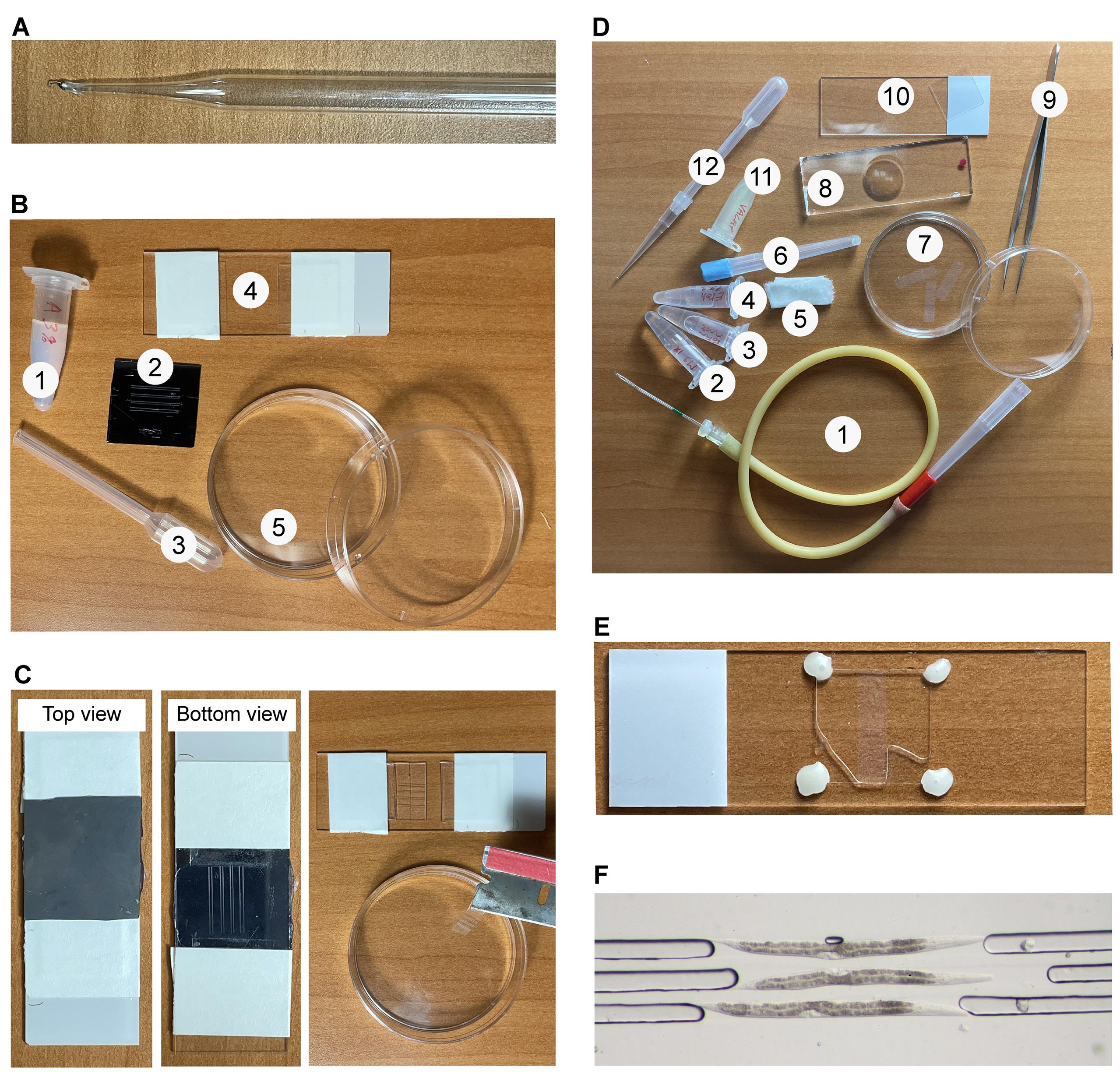
Figure 2. Overview of the materials required and the mounting method. A. Worm pick made of a glass Pasteur pipette and a platinum wire. B. Materials for agarose patterning: 1. 3% agarose solution; 2. Silicon mold micro-patterned with ridges by lithography; 3. Plastic transfer pipet with cut tip; 4. Microscope slide with two coverslips taped to its surface to act as spacers; 5. Petri dish filled with dH2O for storing molded agarose pads. C. Method for preparing agarose pads patterned with grooves. An image of the silicon mold, balanced between two coverslips and pressed against the molten agarose is shown in top (left) and underside (middle) views. The patterned agarose pad is then cut into slices with a single-edge razorblade and the slices are transferred into a Petri dish filled with water (right). D. Materials for mounting worms: 1. Mouth pipette assembled with a microcapillary pipette; 2. M9 buffer; 3. 0.04% Tetramisole in M9; 4. 75% EtOH (for cleaning the microcapillary on the mouth pipette); 5. Blotting paper and Kimwipes cut into ~3 cm strips; 6. Worm eyelash pick; 7. Petri dish filled with water containing the agarose pad slices; 8. 1-well glass depression slide; 9. Forceps; 10. Microscope slide and square coverslip; 11. Valap; 12. Plastic transfer pipet with cut tip and assembled with a 200 µL pipette tip; E. Top view of the final preparation – the agarose pad is centered under the coverslip with the grooves facing up (i.e., towards the coverslip), the corners of the coverslip are stabilized by Valap, and the area around the agarose pad under the coverslip is backfilled with 0.04% Tetramisole in M9. F. Close up of three well-mounted L4 larvae, as viewed through a stereomicroscope.
Mounting worms for live imaging
Note: When performing the following steps, every effort should be made to avoid physical contact with the animals and to work quickly, such that imaging can begin within ~5 min of removing worms from feeding plates. These steps have been optimized for late L4 stage larvae, but also work well for L3 larvae and adult animals.
Make a fresh solution of 0.04% tetramisole in M9.
Note: While this mounting approach can immobilize worms without anesthetics, we find that residual body movements, such as muscle twitching and pharyngeal pumping, can obscure subcellular dynamics, and a low dose of anesthetic (0.04% tetramisole) produces more reliable results.
Prepare a glass micropipette by heating its middle over a Bunsen burner flame and pulling gently from both ends once the glass becomes soft. Break the pipette at a length of ~6 cm and gently heat the broken end to smoothen the glass. An ideal pipette will be narrow enough to ensure precise volume control, but wide enough to transfer late L4 animals with minimal contact (i.e., wide enough for them to freely “thrash”) (Figures 2D #1 and 3A).
Melt a tube of Valap (see Recipes) on a heat block set to 65°C.
Transfer 100 μL of 0.04% tetramisole in M9 into the well of a glass depression slide.
Under a stereomicroscope and using a mouth pipet, gently float 2-5 late L4 larvae off the surface of the plate using ~5 μL of M9, and transfer them via mouth pipette into the tetramisole on the depression slide (Figure 3A).
Using the mouth pipette, blow air on the surface of the tetramisole solution to create a “mini-vortex” for ~10 s. Worm thrashing should reduce noticeably (Figure 3B).
Using a razorblade or forceps, place a 3% agarose pad on a clean glass slide with the groove-molded side facing up.
Note: Perform the following steps quickly to prevent the agarose pad and worms from drying out. Remove excess water from the agarose pad using Whatman paper or a Kimwipe and the mouth pipette.
Using a mouth pipette, gently transfer the worms, one at a time, from the depression slide to the agarose pad, as close to the grooves as possible and using as little liquid as possible (Figure 3C).
With the mouth pipette, gently blow air to move the worms until they fall into the desired groove(s). If the worms remain floating rather than falling into the grooves, then too much liquid is present, so remove excess liquid using the mouth pipette and repeat (Figure 3D).
(Optional) If precise placement of worms is desired (e.g., to capture 2-3 larvae within a single field of view), use a worm eyelash pick to gently sweep the worms into position. Minimize physical contact between the worms and eyelash pick, as this can stimulate the touch receptors and cause the worms to move.
Remove any excess liquid using Whatman paper or a Kimwipe (Figure 3E).
Carefully lower a coverslip onto the agarose pad (Figure 3F).
Note: Dropping the coverslip too quickly may damage the worms.
Trim a 200 μL pipette tip, by cutting ~1 cm off the end using a single edge razorblade, and place it on the end of a plastic transfer pipette. Use this to add a small drop of melted Valap to each corner of the coverslip (Figures 2E and 3G).
Note: Avoid adding too much Valap, as this may heat the coverslip. When adding the Valap, avoid lifting the coverslip.
Using a P200 pipetman, slowly backfill the space under the coverslip with ~100 μL of 0.04% tetramisole in M9 (Figure 3H).
Note: Do not overfill the chamber or fill it too fast, as this can cause the coverslip to lift and displace the worms. Check mounted worms under a stereomicroscope to ensure that they are in the grooves and not moving (Figure 2F).
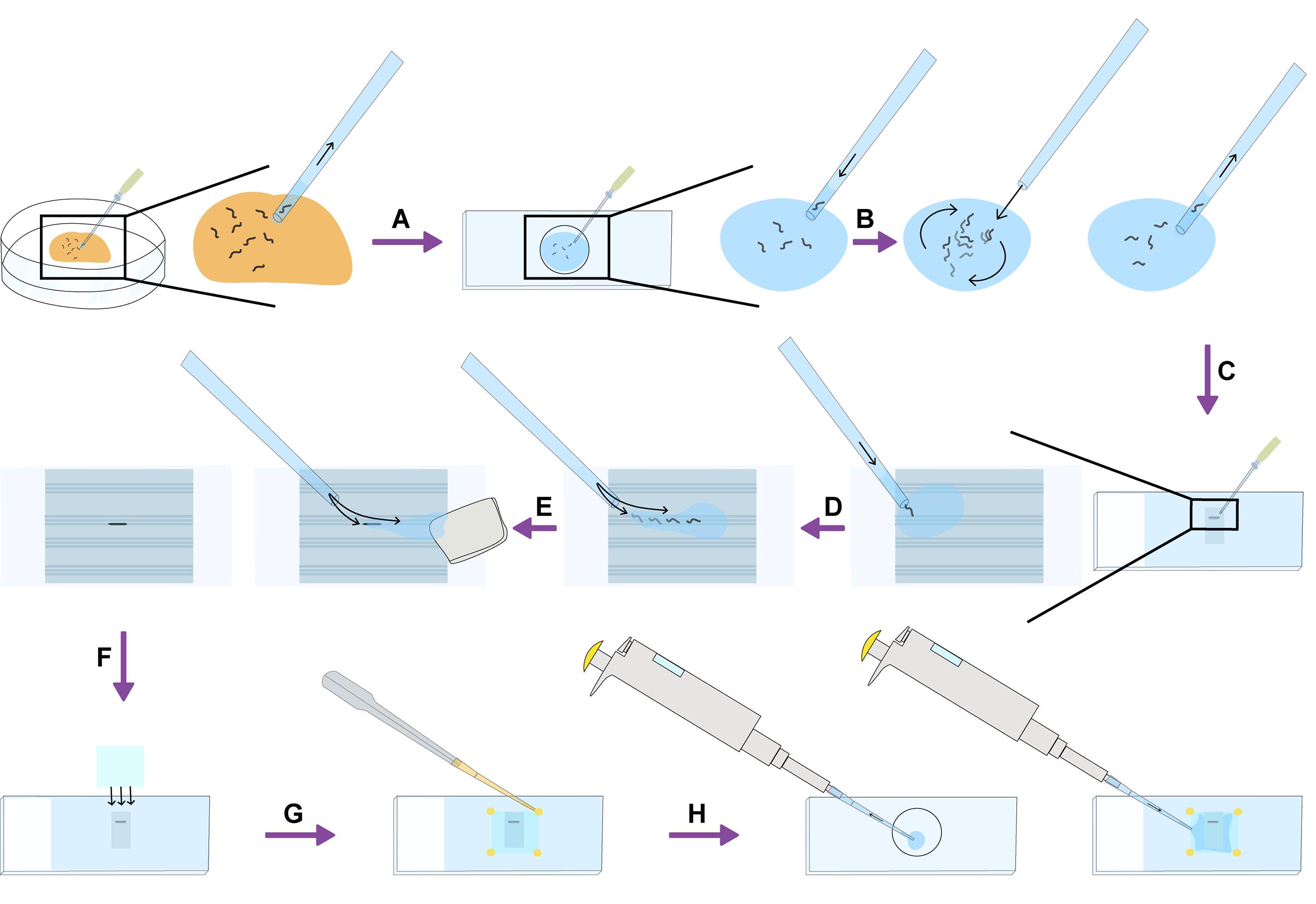
Figure 3. Schematic overview of the mounting procedure. A. C. elegans worms are transferred using a small volume of M9 buffer and a mouth pipette, from a feeding plate to a depression slide filled with 0.04% tetramisole in M9. B. The liquid and worms are then mixed by blowing air on the surface of the liquid using the mouth pipette, to create a “mini-vortex”. C. Individual worms are then transferred by mouth pipette in a small volume of 0.04% tetramisole in M9 to an agarose pad molded with grooves. D. Worms are moved towards the grooves and excess liquid is dispersed using the mouth pipette to blow air across the surface of the liquid in the desired direction. E. Once worms are positioned in the grooves, excess liquid is removed using Whatman paper or a Kimwipe, with the help of the mouth pipette if needed. F. A coverslip is then carefully placed on top of the agarose pad. G. The coverslip is fixed in place by adding a small drop of melted Valap at each corner. H. The area under the coverslip is then backfilled with ~100 μL of the 0.04% tetramisole in M9 remaining in the depression slide.
Imaging
Typical imaging parameters used by our lab to image GSC mitosis are as follows:
Place mounted worms on inverted spinning disk confocal microscope [Zeiss Cell Observer with Yokogawa CSU-X1, using a high NA 63× oil immersion objective (Zeiss 63× Plan-Apochromat DIC (UV) VIS-IR)].
Set laser intensity to 10% of maximum (35 mW 488 nm and 50 mW 561 nm lasers) and exposure time to 200 ms. Set camera (Zeiss Axio Cam 506 Mono) binning to 3 × 3, for a final pixel size of 0.1802 μm.
Set the z-stack step size to 0.5 μm, with sufficient range to encompass the height of the distal germline (typically 20 μm).
Image every 30 s for up to 40 min. After ~40 min of starvation, which is an unavoidable consequence of our mounting method, we observe a significant decrease in the number of GSCs entering mitosis, suggesting that cell and/or organismal physiology changes past this point (Videos 1 and 2; Zellag et al., 2021). As a result, we do not recommend imaging for longer durations.
Note: These imaging parameters were adjusted to minimize the adverse effects of laser exposure and are specific to our microscope. We recommend that users optimize their imaging parameters using the following criteria as benchmarks: (1) A fairly consistent number of cells entering mitosis throughout a 30-40 min acquisition (Figure 4K); (2) An average of 13 mitotic entries per germline (Figure 4I), within a 40 min acquisition; and (3) An average duration of mitosis (as defined below) of ~5 min (Figure 4J).
 Video 1. Mitotic C. elegans GSCs in a late L4 larval germline over a 90-min image acquisition with centrosomes and rachis marked.
Time-lapse movie of the distal end (left) of a gonad from a late L4 worm expressing mNG::ANI-1 (green; rachis) and mCH::β-tubulin (magenta; centrosomes) in the germline. Images were acquired every 30 s for 90 min, with an AxioCam 506 Mono camera (Zeiss) mounted on an inverted Cell Observer spinning-disk confocal microscope (Zeiss; Yokogawa), using a 60x Plan Apochromat DIC (UV) VIS-IR oil immersion objective (Zeiss), controlled by Zen software (Zeiss). A maximum intensity projection of 38 z-sections (0.5 µm sections) is shown. Images were adjusted for brightness and contrast using Fiji (Schindelin et al., 2012). Scale bar = 10 µm. Time stamp is in hour:min. Movie plays at 10 frames per second.
Video 2. Mitotic C. elegans GSCs in a late L4 larval germline over a 40-min image acquisition with centrosomes and chromatin marked.Time-lapse movie of the distal end (left) of a gonad from a late L4 worm expressing GFP::β-tubulin (green; centrosomes) and mCH::Histone H2B (magenta; chromatin) in the germline. Acquisition settings were the same as for Video 1, except for acquisition duration, which was 40 min. A maximum intensity projection of 38 z-sections (0.5 µm sections) is shown. Images were adjusted for brightness and contrast using Fiji (Schindelin et al., 2012). Scale bar = 10 µm. Time stamp is in min:sec. Movie plays at 10 frames per second.
Image processing
The following steps are further detailed in the ReadMe file of our GitHub repository and can be applied to a single movie or several movies in batch mode, if grouped in the same folder.
Registration
Use the ImageJ macro automatedregistrationtool to manually track the spindle midpoint of one or a series of mitotic cells over the duration of the movie (Figure 4A).
Note: Users may track objects other than the spindle midpoint, if other marked structures that follow global sample movement are visible.
Use the Jupyter notebook batchmode movie registration module to generate an x-y translation matrix and to correct the movie accordingly (Figure 4B).
Kymographs in Figure 4B show the correction of sample movement after x-y registration.
Centrosome tracking
Use the ImageJ macro automatedfixhyperstack to restore pixel scaling and frame rate in the registered movie, to crop the borders generated by registration, and perform spot detection and track creation using TrackMate (Tinevez et al., 2017) (Figure 4C). For reference, our TrackMate parameters are as follows: blob diameter = 2.5 μm; linking max distance = 2.7 μm; max frame gap = 2.
Note: TrackMate can identify and track centrosomes marked by fluorescent proteins other than β-tubulin, in cell types other than GSCs, and in organisms other than C. elegans. TrackMate parameters should be optimized by the user based on their sample and imaging parameters, to detect the largest number of true centrosome tracks possible. Spurious tracks are generally removed by the next step.
Centrosome track pairing
Use the Jupyter notebook batchmode track pair classification module to pair spot tracks into likely centrosome track pairs (i.e., centrosomes within the same cell) (Figure 4D).
Note: Our track pair classifier was trained on a large dataset of wild-type C. elegans GSCs. Users who wish to pair centrosomes from other cell types and/or other organisms may need to train their own model. Instructions on how to do this can be found on our GitHub repository.
Scoring mitosis
Use the Matlab script Step1_import_textfile_and_align_cent_tracks to import the xyzt coordinates for paired tracks and to generate a file containing the corresponding midpoint coordinates for each pair (Figure 4E).
Use the ImageJ macro Step2_CropCells to generate cropped maximum intensity projections centered on the midpoint coordinates calculated in Step1 (Figure 4F).
Use the Matlab script Step3_score_mitosis to plot spot-to-spot distance (hereafter “spindle length”) for each predicted pair of centrosomes. This step allows users to exclude false-positive pairs and to score mitotic events [e.g., nuclear envelop breakdown (NEBD), which occurs concomitantly with a rapid decrease in spindle length, and anaphase onset (AO), when spindle length starts to increase rapidly], by clicking on the plot. If the graph is unclear, an option allows the user to view the corresponding cropped tif (Figure 4G).
Use the Matlab script Step4_calc_fits to calculate the duration of mitosis and to extract various mitotic features, including spindle length and anaphase elongation rate. Other features, such as spindle angular displacement or length fluctuations, can readily be calculated from the resulting data. We define “mitosis” as the period of time post-NEBD, once spindle length has reached a ~constant minimum, until AO (Figure 4G); this will encompass most of prometaphase and all of metaphase.
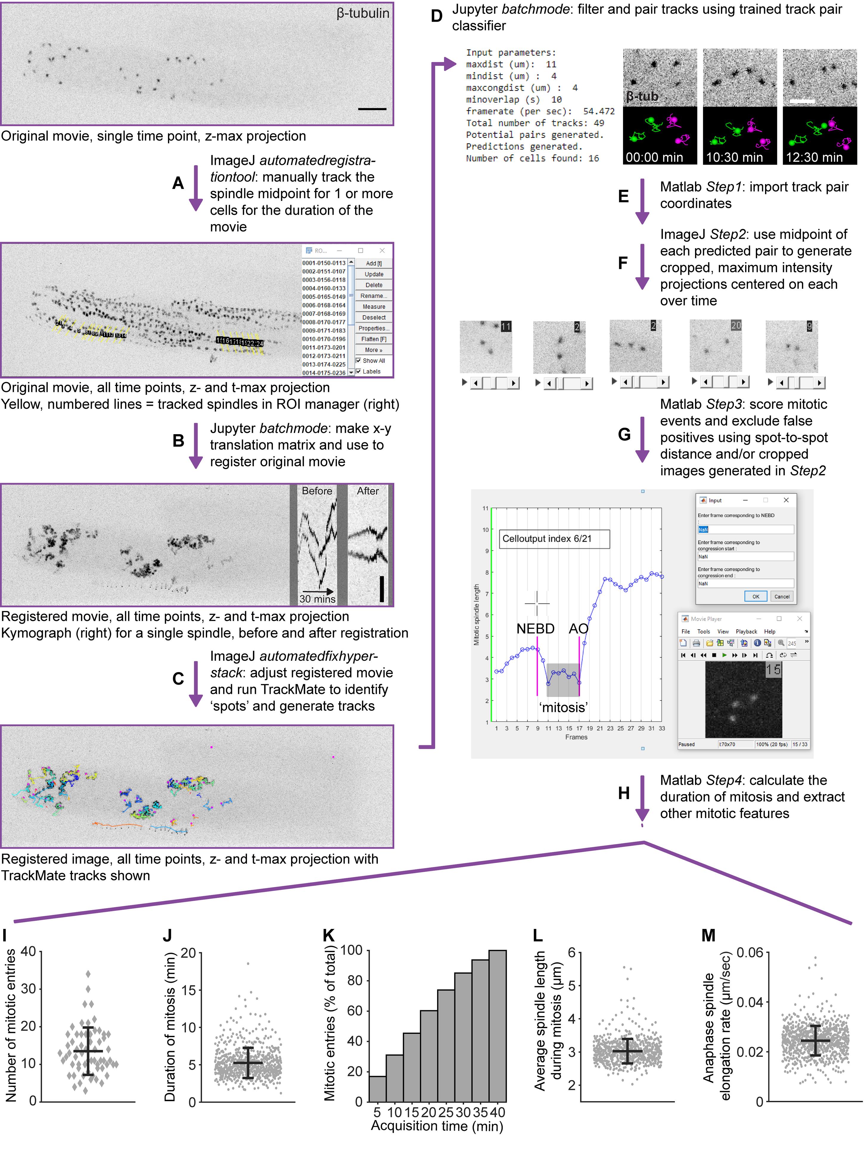
Figure 4. Overview of image processing for analyzing GSCmitotic spindle dynamics in 3D in late L4 larvae. A. To correct for sample movement in x-y, the spindle midpoint of one or more cells is manually tracked over the duration of a maximum intensity projection of the raw/original movie, using the ImageJ macro automatedtegistrationtool. Scale bar = 10 µm. B. Running the movie registration module in the Jupyter notebook batchmode creates an x-y translation matrix from the coordinates of the tracked spindle midpoints and registers the raw/original movie accordingly. Generated using the KymographBuilder plugin in ImageJ (Mary et al., 2016), a kymograph along a ~8 µm-wide line scan through the spindle midpoint of a single GSC over 30 min is shown to illustrate the effectiveness of this correction, before (left) and after (right) x-y registration. Scale bar = 5 µm. C. The ImageJ macro automatedfixhyperstack restores pixel scaling and frame rate, crops the borders generated by registration, and allows the user to perform spot detection and track creation on the registered image using TrackMate (Tinevez et al., 2017). Tracks are shown as colored lines, including bona fide centrosome tracks and spurious tracks. D. TrackMate tracks are then paired by running the track pair classifier module in the Jupyter notebook batchmode. An optimal outcome is shown on the left, where four centrosome tracks from two neighboring cells have been correctly paired (green and magenta tracks) over the course of both divisions. E. The xyzt coordinates for paired spots are imported into Matlab and the midpoint for all pairs is calculated using the script Step1_import_textfile_and_align_cent_tracks. F. The midpoint coordinates are then used by the ImageJ macro Step2_CropCells to generate cropped maximum intensity projections for each pair, with the frame number shown at the upper right-hand corner G. Users can then exclude false positive pairs and score mitotic events, by either clicking on a displayed plot of spot-to-spot distance (i.e., spindle length) over time (left), or by entering timepoints manually after viewing the cropped image generated in F (right) using the Matlab script Step3_score_mitosis. NEBD = nuclear envelop breakdown. AO = anaphase onset. H. The Matlab script Step4_calc_fits calculates the duration of ‘mitosis’ (which we define as illustrated by the shaded box in G) and extracts different mitotic features. I. Number of GSCs entering mitosis (undergoing NEBD) per gonad during the first 40 min of image acquisition from 61 animals [mean ± standard deviation (SD) = 13.5082 ± 6.2786 mitotic entries]. J. Duration of mitosis for 649 cells from 74 animals (mean ± SD = 5.2512 ± 2.0175 min). K. Mitotic entries as a percent of the total number of mitoses during 40 min image acquisition, binned by 5-min intervals relative to acquisition start (n = 61 and 875 mitotic entries). L. Average spindle length during mitosis for 649 cells from 74 animals (mean ± SD = 3.0246 ± 0.3678 µm). M. Spindle elongation rate during early anaphase (First 2 min following anaphase onset) for 819 cells from 74 animals (mean ± SD = 0.0245 ± 0.0059 µm/sec). In I-M, black bars show the mean and error bars represent the SD. Data from three strains (UM679, JDU19, and ARG16, see Table 1) were combined.
Data analysis
The CentTracker image registration module corrects x-y sample movement. However, large and abrupt sample movements in z can lead to untrackable frames and to spot duplications, which can significantly impact the automated pairing module. Therefore, we exclude movies that exhibit severe z-movement. This does not include normal z-drift, which is progressive and has a minimal impact on spot detection and track creation. Typically, severe z-movement occurs when animals are not well situated in their grooves and can be avoided almost entirely by good mounting.
The cell scoring step (J) is crucial for detecting false-positive centrosome pairs when using CentTracker. Spot-to-spot distance plots for true positive centrosome pairs have a consistent pattern (Figure 4G), so false-positive plots should be readily identifiable. However, we recommend viewing the corresponding cropped tif for any unusual plots, especially if the GSCs under analysis are not wild-type, and/or are expected to have spindle defects.
The mitotic parameters displayed in Figure 4 are for GSCs from late L4 larvae and were calculated as described in Zellag et al. (2021), where details for the extraction of additional mitotic features can also be found. The total number of mitotic entries per gonad was determined using manual track pairing, not the track pair classifier in CentTracker, which has a discovery rate of ~80% in wild-type animals (Zellag et al., 2021).
Notes
The silicon mold used in this protocol is etched to form positive bands 26 μm high and 50 μm wide and generates v-shaped grooves of the same proportions, with angled walls (Figure 1B). A simple photomask design can be created using computer-aided design (CAD) software, and the photomask production and photolithography can be achieved at most microfabrication facilities. We have subsequently found that square-shaped grooves (Figure 1B) produce similar and even potentially better results, and may be less challenging/costly for the photolithography step. We have tested the following designs and all of them are adequate for mounting:
For mid to late L3 worms: Square-shaped grooves 20 μm deep and 20 μm wide.
For Late L4 worms: Square-shaped grooves 35 μm deep and 38-43 μm wide.
For 1 day-old adult worms: Square-shaped grooves 55 μm deep and 60-65 μm wide.
If microfabrication facilities are not available, using a vinyl Long Play (LP) record as a mold (Zhang et al., 2008; Rivera Gomez and Schvarzstein, 2018) can yield reasonably good results (Zellag et al., 2021).
Make a worm eyelash pick using a human eyelash or a cat whisker. Hold the eyelash/whisker with a pair of fine-tipped tweezers and insert the root end into the end of a 200 μL pipette tip, which is filled with molten Valap. Once the Valap solidifies, the eyelash/whisker should stay in place. Alternatively, the end of ~1,000 μL pipet tip can be melted, and the eyelash/whisker inserted while the plastic is still malleable (Figure 2D).
Recipes
M9 buffer (1,000 mL)
3 g KH2PO4
6 g Na2HPO4
5 g NaCl
1 mL of 1 M MgSO4
dH2O to bring final volume to 1,000 mL
Combine all ingredients until dissolved and sterilize by filtration using a 0.2 μm pore size.
Valap
1:1:1 by weight Vaseline, lanolin, and paraffin
Combine all ingredients in a glass beaker on a hot plate set at a low temperature. Stir occasionally until melted and homogenous. Store at room temperature as ~1 mL aliquots.
Bleaching solution (5 mL)
1 mL of commercial bleach (~10% available chlorine)
250 μL of 10M NaOH
3.75 mL of dH2O
Add bleach and NaOH to water in a 15 mL conical tube. Makes enough to bleach five 60 mm plates of gravid adults. Make fresh every time, ideally within 1 h of use. Do not store.
Note: As bleach degrades over time, we recommend using bottles of commercial bleach with a known and fairly recent (within 1 year) purchase date.
2% w/v Tetramisole solution
Make a 2% w/v solution in dH2O, store at 4°C and dilute to 0.04% in M9 buffer before use.
3% w/v volume Agarose powder solution
Make a 3% w/v volume solution in dH2O.
Acknowledgments
We thank Dr. Jean-Claude Labbé (JCL) of IRIC for advice and critical reading of this manuscript. We also thank Drs. Amy Maddox (UNC Chapel Hill), Arshad Desai (UC, San Diego), Benjamin Lacroix (Institut Jacques Monod) for sharing strains, IRIC's Bio-imaging facility and McGill’s Advanced BioImaging Facility (ABIF) for technical assistance, and members of the Labbé and Gerhold labs for help and advice. RMZ held an Alexander Graham Bell Canada Graduate Scholarship from the Natural Sciences and Engineering Research Council of Canada (NSERC) and an IRIC Doctoral Scholarship. YZ was partially supported by the Sheila Ann MacInnis Grant Science Undergraduate Research Award (SURA). This work was funded by grants from the Canadian Institutes of Health Research (PJT-153283 to JCL and ARG and PJT-159523 to ARG).
This protocol was part of and derived from Zellag et al. (2021).
Competing interests
There are no conflicts of interest or competing interests.
References
- Angelo, G. and Van Gilst, M. R. (2009). Starvation protects germline stem cells and extends reproductive longevity in C. elegans. Science 326(5955): 954-958.
- Amini, R., Goupil, E., Labella, S., Zetka, M., Maddox, A. S., Labbé, J. C. and Chartier, N. T. (2014). C. elegans Anillin proteins regulate intercellular bridge stability and germline syncytial organization. J Cell Biol 206(1): 129-143.
- Brenner, S. (1974). The genetics of Caenorhabditis elegans. Genetics 77(1): 71-94.
- Baugh, L. R. and Sternberg, P. W. (2006). DAF-16/FOXO regulates transcription of cki-1/Cip/Kip and repression of lin-4 during C. elegans L1 arrest. Curr Biol 16(8): 780-785.
- Barbosa, J. S., Sanchez-Gonzalez, R., Di Giaimo, R., Baumgart, E. V., Theis, F. J., Götz, M. and Ninkovic, J. (2015). Neurodevelopment. Live imaging of adult neural stem cell behavior in the intact and injured zebrafish brain. Science 348(6236): 789-793.
- Berger, S., Lattmann, E., Aegerter-Wilmsen, T., Hengartner, M., Hajnal, A., deMello, A. and Casadevall I Solvas, X. (2018). Long-term C. elegans immobilization enables high resolution developmental studies in vivo. Lab Chip 18(9): 1359-1368.
- Burnett, K., Edsinger, E. and Albrecht, D. R. (2018). Rapid and gentle hydrogel encapsulation of living organisms enables long-term microscopy over multiple hours. Commun. Biol 1: 73.
- Berger, S. and Spiri, S. (2021). Microfluidic-based imaging of complete Caenorhabditis elegans larval development. Development 148(18).
- Chai, Y., Li, W., Feng, G., Yang, Y., Wang, X. and Ou, G. (2012). Live imaging of cellular dynamics during Caenorhabditis elegans postembryonic development. Nat Protoc 7(12): 2090-2102.
- Dickinson, D. J., Ward, J. D., Reiner, D. J. and Goldstein, B. (2013). Engineering the Caenorhabditis elegans genome using Cas9-triggered homologous recombination. Nature Methods 10(10):1028-1034.
- Fielenbach, N. and Antebi, A. (2008). C. elegans dauer formation and the molecular basis of plasticity. Genes Dev 22(16): 2149-2165.
- Fabig, G., Löffler, F., Götze, C. and Müller-Reichert, T. (2020a). Live-cell Imaging and Quantitative Analysis of Meiotic Divisions in Caenorhabditis elegans Males. Bio-protocol 10(20): e3785.
- Fabig, G., Kiewisz, R., Lindow, N., Powers, J. A., Cota, V., Quintanilla, L. J., Brugués, J., Prohaska, S., Chu, D. S., and Müller-Reichert, T. (2020b). Male meiotic spindle features that efficiently segregate paired and lagging chromosomes.eLife 9: e50988.
- Gray, J. and Lissmann, H. W. (1964). THE LOCOMOTION OF NEMATODES. J Exp Biol 41: 135-154.
- Gerhold, A. R., Ryan, J., Vallée-Trudeau, J. N., Dorn, J. F., Labbé, J. C. and Maddox, P. S. (2015). Investigating the regulation of stem and progenitor cell mitotic progression by in situ imaging. Curr Biol 25(9): 1123-1134.
- Gordon, K. L., Zussman, J. W., Li, X., Miller, C. and Sherwood, D. R. (2020). Stem cell niche exit in C. elegans via orientation and segregation of daughter cells by a cryptic cell outside the niche. eLife 9: e56383.
- Hirsh, D., Oppenheim, D. and Klass, M. (1976). Development of the reproductive system of Caenorhabditis elegans. Dev Biol 49(1): 200-219.
- Hwang, H., Krajniak, J., Matsunaga, Y., Benian, G. M. and Lu, H. (2014). On-demand optical immobilization of Caenorhabditis elegans for high-resolution imaging and microinjection. Lab Chip 14(18): 3498-3501.
- Joshi, P. M., Riddle, M. R., Djabrayan, N. J. and Rothman, J. H. (2010). Caenorhabditis elegans as a model for stem cell biology.Dev Dyn Off Publ Am Assoc Anat 239(5): 1539-1554.
- Kimble, J. E. and White, J. G. (1981). On the control of germ cell development in Caenorhabditis elegans. Dev Biol 81(2): 208-219.
- Kim, E., Sun, L., Gabel, C. V. and Fang-Yen, C. (2013). Long-term imaging of Caenorhabditiselegans using nanoparticle-mediated immobilization. PLoS One 8(1): e53419.
- Luke, C. J., Niehaus, J. Z., O'Reilly, L. P. and Watkins, S. C. (2014). Non-microfluidic methods for imaging live C. elegans. Methods 68(3): 542-547.
- Maddox, A. S., Habermann, B., Desai, A. and Oegema, K. (2005). Distinct roles for two C.elegans anillins in the gonad and early embryo. Development 132(12): 2837-2848.
- Morrison, S. J. and Kimble, J. (2006). Asymmetric and symmetric stem-cell divisions in development and cancer. Nature 441(7097): 1068-1074.
- Magescas, J., Zonka, J. C. and Feldman, J. L. (2019). A two-step mechanism for the inactivation of microtubule organizing center function at the centrosome. eLife 8: e47867.
- Martin, J. L., Sanders, E. N., Moreno-Roman, P., Jaramillo Koyama, L. A., Balachandra, S., Du, X. and O'Brien, L. E. (2018). Long-term live imaging of the Drosophila adult midgut reveals real-time dynamics of division, differentiation and loss. eLife 7: e36248.
- Mary, H., Rueden, C., and Ferreira, T. (2016). KymographBuilder: Release 1.2.4. Zenodo.
- Merritt, C., and Seydoux, G. (2010). Transgenic solutions for the germline. WormBook : The Online Review of C. elegans Biology. 1-21. doi: 10.1895/wormbook.1.148.1.
- Nguyen, P. D. and Currie, P. D. (2018). In vivo imaging: shining a light on stem cells in the living animal. Development 145(7).
- Park, S., Greco, V. and Cockburn, K. (2016). Live imaging of stem cells: answering old questions and raising new ones. Curr Opin Cell Biol 43: 30-37.
- Priti, A., Ong, H. T., Toyama, Y., Padmanabhan, A., Dasgupta, S., Krajnc, M., and Zaidel-Bar, R. (2018). Syncytial germline architecture is actively maintained by contraction of an internal actomyosin corset. Nat Commun 9(1): 4694.
- Rompolas, P., Deschene, E. R., Zito, G., Gonzalez, D. G., Saotome, I., Haberman, A. M. and Greco, V. (2012). Live imaging of stem cell and progeny behaviour in physiological hair-follicle regeneration. Nature 487(7408): 496-499.
- Ritsma, L., Ellenbroek, S. I. J., Zomer, A., Snippert, H. J., de Sauvage, F. J., Simons, B. D., Clevers, H. and van Rheenen, J. (2014). Intestinal crypt homeostasis revealed at single-stem-cell level by in vivo live imaging. Nature 507(7492): 362-365.
- Rivera Gomez, K. A., and Schvarzstein, M. (2018). Immobilization of nematodes for live imaging using an agarose pad produced with a Vinyl Record. MicroPublication Biology 2018(08).
- Rosu, S. and Cohen-Fix, O. (2017). Live-imaging analysis of germ cell proliferation in the C. elegans adult supports a stochastic model for stem cell proliferation. Dev Biol 423(2): 93-100.
- Sulston, J. E. and Horvitz, H. R. (1977). Post-embryonic cell lineages of the nematode, Caenorhabditis elegans. Dev Biol 56(1): 110-156.
- Stiernagle, T. (2006). Maintenance of C. elegans. WormBook. 1-11.
- Schindelin, J., Arganda-Carreras, I., Frise, E., Kaynig, V., Longair, M., Pietzsch, T., Preibisch, S., Rueden, C., Saalfeld, S., Schmid, B., et al. (2012). Fiji: an open-source platform for biological-image analysis. Nat Methods 9(7): 676-682.
- Timmons, L. and Fire, A. (1998). Specific interference by ingested dsRNA. Nature 395(6705): 854.
- Tinevez, J. Y., Perry, N., Schindelin, J., Hoopes, G. M., Reynolds, G. D., Laplantine, E., Bednarek, S. Y., Shorte, S. L. and Eliceiri, K. W. (2017). TrackMate: An open and extensible platform for single-particle tracking. Methods 115: 80-90.
- Wong, B. G., Paz, A., Corrado, M. A., Ramos, B. R., Cinquin, A., Cinquin, O. and Hui, E. E. (2013). Live imaging reveals active infiltration of mitotic zone by its stem cell niche. Integr Biol (Camb) 5(7): 976-982.
- Yoshida, S., Sukeno, M. and Nabeshima, Y. (2007). A vasculature-associated niche for undifferentiated spermatogonia in the mouse testis. Science 317(5845): 1722-1726.
- Zhou, K., Rolls, M. M. and Hanna-Rose, W. (2013). A postmitotic function and distinct localization mechanism for centralspindlin at a stable intercellular bridge. Dev Biol 376(1): 13-22.
- Zeiser, E., Frøkjær-Jensen, C., Jorgensen, E., and Ahringer, J. (2011). MosSCI and Gateway Compatible Plasmid Toolkit for Constitutive and Inducible Expression of Transgenes in the C. elegans Germline. PloS One 6(5): e20082.
- Zhang, M., Chung, S. H., Fang-Yen, C., Craig, C., Kerr, R. A., Suzuki, H., Samuel, A. D., Mazur, E. and Schafer, W. R. (2008). A self-regulating feed-forward circuit controlling C. elegans egg-laying behavior. Curr Biol 18(19): 1445-1455.
- Zellag, R. M., Zhao, Y., Poupart, V., Singh, R., Labbé, J. C. and Gerhold, A. R. (2021). CentTracker: a trainable, machine-learning-based tool for large-scale analyses of Caenorhabditis elegans germline stem cell mitosis. Mol Biol Cell 32(9): 915-930.
Article Information
Copyright
© 2022 The Authors; exclusive licensee Bio-protocol LLC.
How to cite
Readers should cite both the Bio-protocol article and the original research article where this protocol was used:
- Zellag, R. M., Zhao, Y. and Gerhold, A. R. (2022). Live-cell Imaging and Analysis of Germline Stem Cell Mitosis in Caenorhabditis elegans. Bio-protocol 12(1): e4272. DOI: 10.21769/BioProtoc.4272.
- Zellag, R. M., Zhao, Y., Poupart, V., Singh, R., Labbé, J. C. and Gerhold, A. R. (2021). CentTracker: a trainable, machine-learning-based tool for large-scale analyses of Caenorhabditis elegans germline stem cell mitosis. Mol Biol Cell 32(9): 915-930.
Category
Stem Cell > Germ cell
Developmental Biology > Cell growth and fate
Cell Biology > Cell imaging > Live-cell imaging
Do you have any questions about this protocol?
Post your question to gather feedback from the community. We will also invite the authors of this article to respond.