- Protocols

- Articles and Issues
- For Authors
- About
- Become a Reviewer

Biophysical Characterization of Iron-Sulfur Proteins
Published: Vol 11, Iss 20, Oct 20, 2021 DOI: 10.21769/BioProtoc.4202 Views: 3912
Reviewed by: Manjula MummadisettiRama Reddy GoluguriPallavi Prasad
Original research article
The authors used this protocol in:

Dec 2020
Advertisement


Protocol Collections
Comprehensive collections of detailed, peer-reviewed protocols focusing on specific topics


Abstract
Iron-sulfur proteins are primordial catalysts and biological electron carriers that today drive major metabolic pathways across all forms of life. They can access a diversity of oxidation states and can mediate electron transfer over an extended range of reduction potentials spanning more than 1 V. Depending on the protein micro-environment and geometry of ligand, co-ordination the iron-sulfur clusters can occur in different forms [2Fe-2S], [3Fe-4S], HiPIP [4Fe-4S], and [4Fe-4S]. There are several spectroscopic methods available to characterize the composition and electronic configuration of the iron-sulfur clusters, such as optical methods and electron paramagnetic resonance. This paper presents the protocols used to characterize the metal center of Coiled-Coil Iron-Sulfur (CCIS), an artificial metalloprotein containing one [4Fe-4S] cluster. It is expected that these protocols will be of general utility for other iron-sulfur proteins.
Keywords: Iron-sulfur proteinsBackground
Iron-sulfur proteins are of ancient origin, first evolving several billion years ago. They are ubiquitous today, found among all domains of life (Beinert, 2000; Camprubi et al., 2017). These proteins drive almost all major metabolic pathways such as photosynthesis, respiration, nitrogen fixation, methanogenesis, and hydrogen metabolism (Fontecave, 2006; Shaw et al., 2013; Einsle, 2014; Gnandt et al., 2016; Wagner et al., 2016; Lubitz et al., 2019). These proteins function mainly as electron shuttles, routing electrons to the active sites of redox-active enzymes (Johnson et al., 2005; Cordes and Giese, 2009). Furthermore, iron–sulfur proteins are also involved in non-redox functions, such as aconitase, which senses low iron concentrations within cells (Flint and Allen, 1996; Beinert and Kiley, 1999). There are several common cluster compositions, including [2Fe-2S], [3Fe-4S], and [4Fe-4S]. Due to this chemical diversity, they can mediate the transfer of electrons over an extended range between +500 and -680 mV (Kyritsis et al., 1998; Brzoska et al., 2006; Liu et al., 2014).
In this paper, we describe protocols to characterize iron-sulfur proteins using Coiled-Coil Iron-Sulfur (CCIS), an artificial protein [4Fe-4S]-binding protein as a case study (Jagilinki et al., 2020). The CCIS/pET-28a (+) DNA plasmid has been commercially procured (GenScript, USA) [refer toGrzyb et al. (2010) andJagilinki et al. (2020) for the amino acid sequence of the CCIS protein]. The molecular weight of CCIS is 11.6 kDa, and its extinction coefficient at 280 nm is 16,500 (M-1cm-1). [4Fe-4S] clusters are highly sensitive to oxygen and require completely anaerobic conditions to study and characterize them (Imlay, 2006). Anaerobic conditions can be maintained in the lab using an anaerobic chamber with 95% nitrogen and 5% hydrogen. The presence of metal ions within the protein enables them to be characterized by several additional biophysical techniques, such as UV-Vis spectroscopy, Electron Paramagnetic Resonance (EPR), and Inductively coupled plasma atomic emission spectroscopy (ICP-AES). The protocols that follow are examples of relevant biochemical and biophysical methods to characterize CCIS and related molecules, specifically UV-visible absorption spectroscopy, Circular Dichroism (CD), thermal denaturation (both secondary structure and [4Fe-4S] cluster), Electron Paramagnetic Resonance (EPR), and Inductively coupled plasma atomic emission spectroscopy (ICP-AES).
Materials and Reagents
Centricon® centrifugal filters (Millipore, catalog number: UFC801024)
1.7 ml Eppendorf tubes (VWR, catalog number: 87003-294)
Pyrex test tubes (VWR, catalog number: 60815-104)
1 cm cuvettes with airtight caps for UV and CD (Hellma, catalog number: 117200F-10-40)
1 mm cuvettes with airtight caps for CD (Hellma, catalog number: 110-1-40)
4 mm quartz EPR tubes (Wilmad, catalog number: 707-SQ-250M)
Rubber caps for EPR tubes (McMaster, part number: 92805K7)
PD 10 Desalting Columns (GE, catalog number: GE17-0851-01)
Tris-base (J.T. Baker, catalog number: 410901)
Sodium chloride (NaCl) (Sigma-Aldrich, catalog number: S9888)
Glycerol (Sigma-Aldrich, catalog number: G6279)
Liquid helium for EPR experiments
Nitric acid (HNO3) (Sigma-Aldrich, catalog number: 225711)
Iron Standard for ICP (Millipore, catalog number: 43149)
Sulfur Standard for ICP (Millipore, catalog number: 18021)
Copper(II) sulfate pentahydrate (CuSO4·5H2O) (Sigma-Aldrich, catalog number: 203165)
1 M Sodium dithionite (Na2S2O4) (Merck, catalog number: 1065070500) (see Recipes)
Buffer A (see Recipes)
Buffer B (see Recipes)
Buffer C (see Recipes)
Equipment
Sorvall centrifuge (Thermo Scientific, model: Sorvall LYNX 6000, catalog number: 75006590)
Mini-Centrifuge (Eppendorf, Minispin, catalog number: 22620100)
pH meter (Hanna, Edge pH meter, catalog number: HI2002-01)
NanoDrop (Denovix, model: DS-11 FX+)
UV-visible spectrophotometer (Jasco, model: V-7200 Spectrophotometer, catalog number: V-7200)
CD spectrometer (Applied Photophysics, Chirascan-plus, catalog number: V100)
EPR machine (Bruker, model: ELEXSYS-E580e, catalog number: E580)
Water bath (Fisher Scientific, Isotemp, catalog number: 205 FS-205)
ICP-AES (Agilent, model: ICP-OES 5110, catalog number: 5110)
Anaerobic chamber filled with N2/H2 (95%/5%) (Coy lab, Vinyl anaerobic chamber, catalog number: Type A)
Rectangular EPR resonator (Bruker 4102ST)
Oxford helium-flow cryostat (ESR900)
Software
Spectra Manager Suite (provided by Jasco for V-7200 Spectrophotometer)
Chirascan Q100 Software (provided by Applied Photophysics for Chirascan-plus V100 CD spectrometer)
Xepr software (provided by Bruker for ELEXSYS-E580e EPR machine)
Igor Pro for data analysis (License required from www.wavemetrics.com )
Procedure
The following methods describe sample preparation and experimental setup needed to perform UV-visible absorption, CD, thermal denaturation (both secondary structure and [4Fe-4S] cluster), EPR, and ICP-AES. These protocols have been successfully demonstrated on the CCIS protein and helix-1 of CCIS (Jagilinki et al., 2020). These methods can be used in general for any natural and artificial [4Fe-4S]-binding proteins.
UV-visible spectroscopy
Switch on the UV-visible spectrophotometer.
Open the spectra manager suite and under the settings tab, update the following information: Start, 800 nm; stop, 260 nm; average time, 0.1 sec; data interval, 1 nm; and scan rate, 600 nm/min.
Add 1-2 ml of buffer A into a 1 cm path quartz cuvette and record the background blank spectrum between 800 and 260 nm.
Add 1-2 ml of 100-200 µM holo-CCIS in buffer A into a 1 cm path quartz cuvette (Figure 1A) and seal with an airtight cap inside the anaerobic chamber; transfer the cuvette into the UV-visible spectrometer.
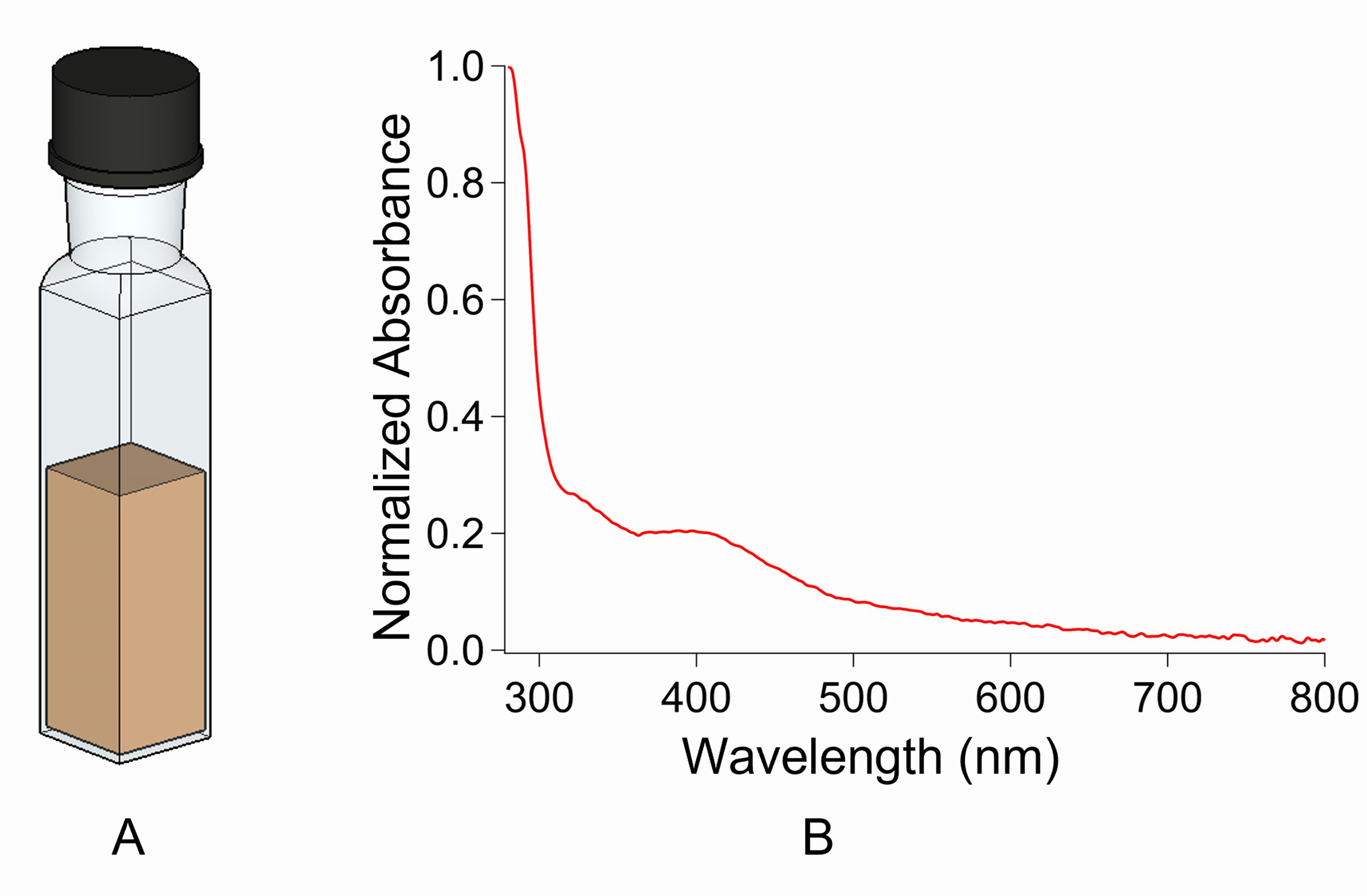
Figure 1. Airtight cuvette for UV-visible spectroscopy. A. A 1 cm path length quartz cuvette with airtight cap for performing UV and CD in visible region. B. UV-visible spectra of CCIS protein.Record the spectra between 800 and 260 nm, subtracting the buffer A spectrum from the sample spectrum.
Typical [4Fe-4S] spectra contain a significant peak with absorbance maxima between 395 and 400 nm and a characteristic shoulder between 320 and 360 nm (see Note 1). Refer to Figure 3(A) inset in Jagilinki et al. (2020) or Figure 1B.
Turn off the UV-visible spectrophotometer.
CD spectroscopy in far UV
Before switching on the CD spectrometer, turn the nitrogen flow into the CD spectrometer and let it purge for at least 30 min.
During this time, exchange the protein buffer to buffer B using a PD-10 column (see Note 2).
Cut the bottom tip of the PD-10 column and drain off the liquid from the column through gravity flow inside the anaerobic chamber.
Pass 50 ml of buffer B to equilibrate the column, then load 2.5 ml of protein and allow it to enter the PD-10 column.
Then, intermittently add 1 ml of buffer B and start collecting protein from 3 ml to 6 ml.
If the protein concentration is higher and more than required, dilute with buffer B until the concentration reaches 10-20 µM.
Switch on the CD spectrometer and set the following parameters in the Chirascan Q100 Software: bandwidth, 1 nm, and digital integration time, 2 s. Ensure that there is an uninterrupted flow of nitrogen into the CD spectrometer throughout the duration of the experiment.
Add 200-300 µl of buffer B into a 1 mm path quartz cuvette and record the background blank spectrum between 250 and 195 nm.
Add 200-300 µl of 10-20 µM protein into a 1 mm path quartz cuvette and seal with an airtight cap inside the anaerobic chamber; transfer the cuvette into the CD spectrometer.
Record the spectrum between 250 and 195 nm, subtracting the blank spectrum.
Record the spectra for both holo and apo forms of the protein (see Note 3).
A typical far UV spectrum of α-rich helical proteins contains two prominent negative bands at 222 and 208 nm (see the traces in Figure 2A), whereas a typical far UV spectrum of β-rich proteins has one major broad dip between 215 and 218 nm.
After performing the CD experiments, close the CD program and turn off the CD spectrometer. Allow the nitrogen inflow into the CD spectrometer for another 15 min, before turning off the nitrogen flow.
To convert the CD values into Mean Residue Ellipticity, use the following equation:
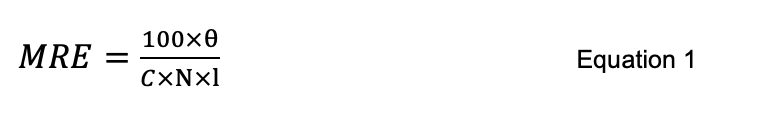
where,
MRE stands for Mean Residue Ellipticity,
(θ) is the ellipticity in degrees,
C is the molar protein concentration,
N is the number of amino acids in the protein,
l is the optical path length in cm.
CD spectroscopy in visible region
Before switching on the CD spectrometer, turn the nitrogen flow and purge it for at least 30 min.
Add 1-2 ml of buffer B into a 1 cm path quartz cuvette and record the background blank spectrum between 800 and 300 nm.
Add 1-2 ml of 200 µM protein into a 1 cm path quartz cuvette (Figure 1A) and seal with an airtight cap inside the anaerobic chamber; transfer the cuvette into the CD spectrometer.
Record the spectrum between 800 and 300 nm subtracting the blank spectrum (see Note 4).
A typical [4Fe-4S] CD spectrum in the visible region contains two significant troughs at approximately 360 nm and 550 nm and a characteristic crest between 430 and 440 nm (see the traces in Figure 2B). For CD spectra in the visible region for other types of clusters, refer to Freibert et al. (2018) .
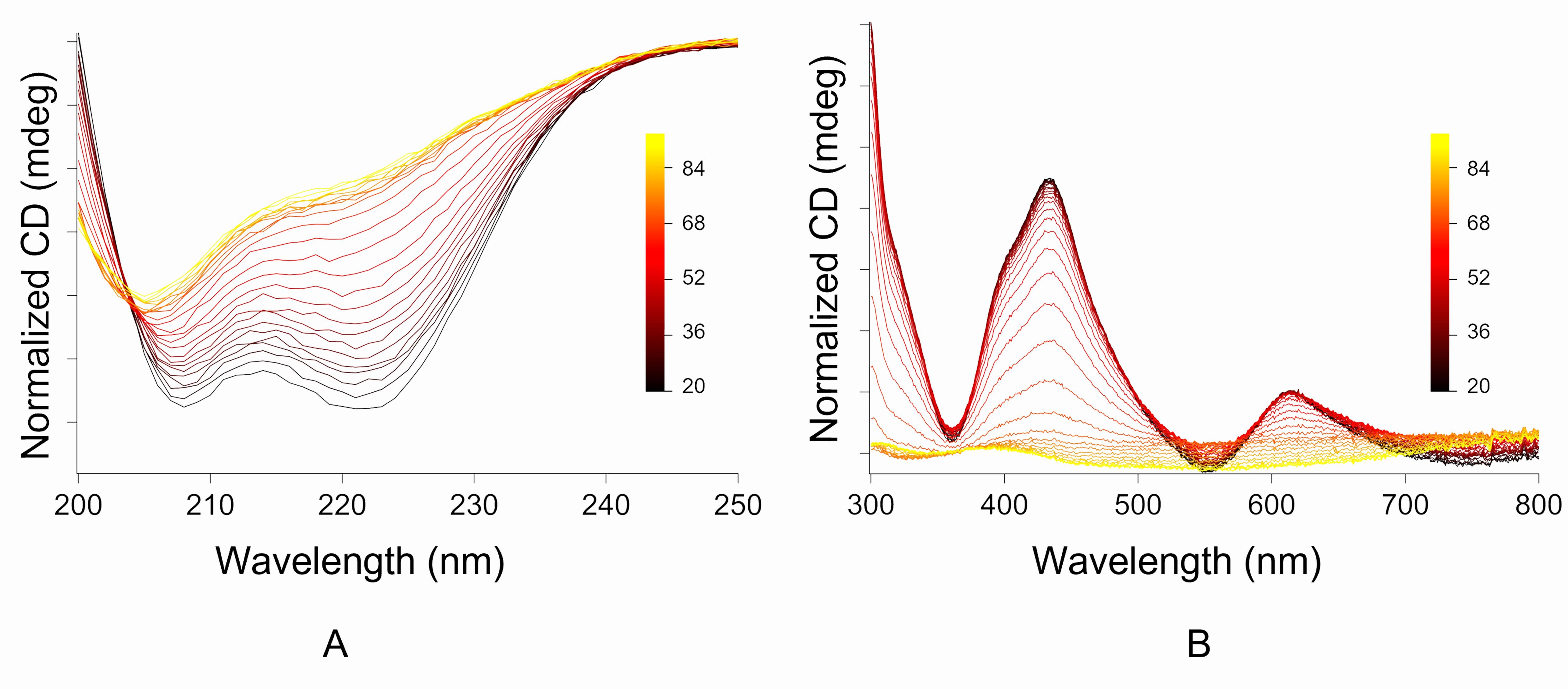
Figure 2. Thermal denaturation profiles. A. Thermal denaturation profile of helix-1 of CCIS in the far UV region to determine the thermal stability of the secondary structure of the protein. B. Thermal denaturation profile of helix-1 of CCIS in the visible region to determine the thermal stability of the [4Fe-4S] cluster.
Thermal denaturation using CD spectroscopy in far UV
After recording the CD spectrum in the far UV region, as mentioned in section B, initiate the thermal kinetics program within the CD operational software.
Set the temperature range between 20 and 90°C with intermittent steps of 2°C between scans. Allow the sample to incubate for at least 5 min at each temperature.
Start the thermal denaturation program. Record for both holo and apo forms of the protein individually (see Note 5).
Select a specific wavelength from the above experiment (222 nm for α-helical proteins or 218 nm for β-sheet proteins) and plot a trace against the temperature on the X-axis to determine the melting temperature (Tm) of the protein (see Note 6).
Thermal denaturation using CD spectroscopy in the visible region
After recording the CD spectrum in the visible region, as mentioned in section C, initiate the thermal kinetics program within the CD operational software.
Set the temperature range between 20 and 90°C with with an increment of 2°C between scans. Allow the sample to incubate for at least 12 min at each temperature (see Note 7).
Start the thermal denaturation program. Perform the experiment only for the holo-protein.
Select a specific wavelength from the above experiment (typically between 400 and 450 nm) and plot a trace against the temperature on the X-axis to determine the melting temperature (Tm) of the iron–sulfur cluster within the protein (see Note 6).
Iron-sulfur cluster identification within the CCIS by EPR
Iron-sulfur cluster in its resting redox state, [4Fe-4S]2+, is diamagnetic and EPR-silent. For EPR characterization, the iron-sulfur clusters are reduced to paramagnetic state [4Fe-4S]1+ using sodium dithionite (Na2S2O4) (see Note 8).
Prepare two EPR samples in the anaerobic chamber: one in the resting state [4Fe-4S]2+ and the second in the dithionite-reduced state [4Fe-4S]1+. For each sample, use 200 µl of 200 µM holo-CCIS in buffer C (see Note 9). For the dithionite-reduced sample, add 8-10 µl of 1 M sodium dithionite (Na2S2O4).
Mix the solution properly in an eppendorf tube and transfer the resting and reduced state samples into clean EPR quartz tubes; seal the open end of the tubes with an airtight rubber cap.
Take out the EPR tube from the anaerobic chamber and immediately freeze in liquid nitrogen. Keep the samples frozen at all times.
Record the continuous-wave (cw) EPR spectra of the reduced and resting state samples at 10-30 K using a rectangular EPR resonator (Bruker 4102ST) and Oxford helium-flow cryostat (ESR900).
Apply the following experimental conditions: microwave power, 0.2-2 mW, and modulation amplitude, 1-2 mT.
Confirm absence of any EPR signal for the holo-protein sample in its resting redox state, [4Fe-4S]2+.
A typical EPR spectrum of sodium dithionite reduced [4Fe-4S]1+ protein exhibits an axial EPR line shape consisting of two major peaks and showing up at magnetic fields corresponding to g|| (g1) with average values between 2.08 and 2.04 and g⊥ (g2,g3) with average values between 1.94 and 1.90. Refer to Figure 3(B) by Jagilinki et al. (2020) or Figure 3. For EPR spectral properties of other types of iron-sulfur clusters, refer to Bertini et al. (1995) .
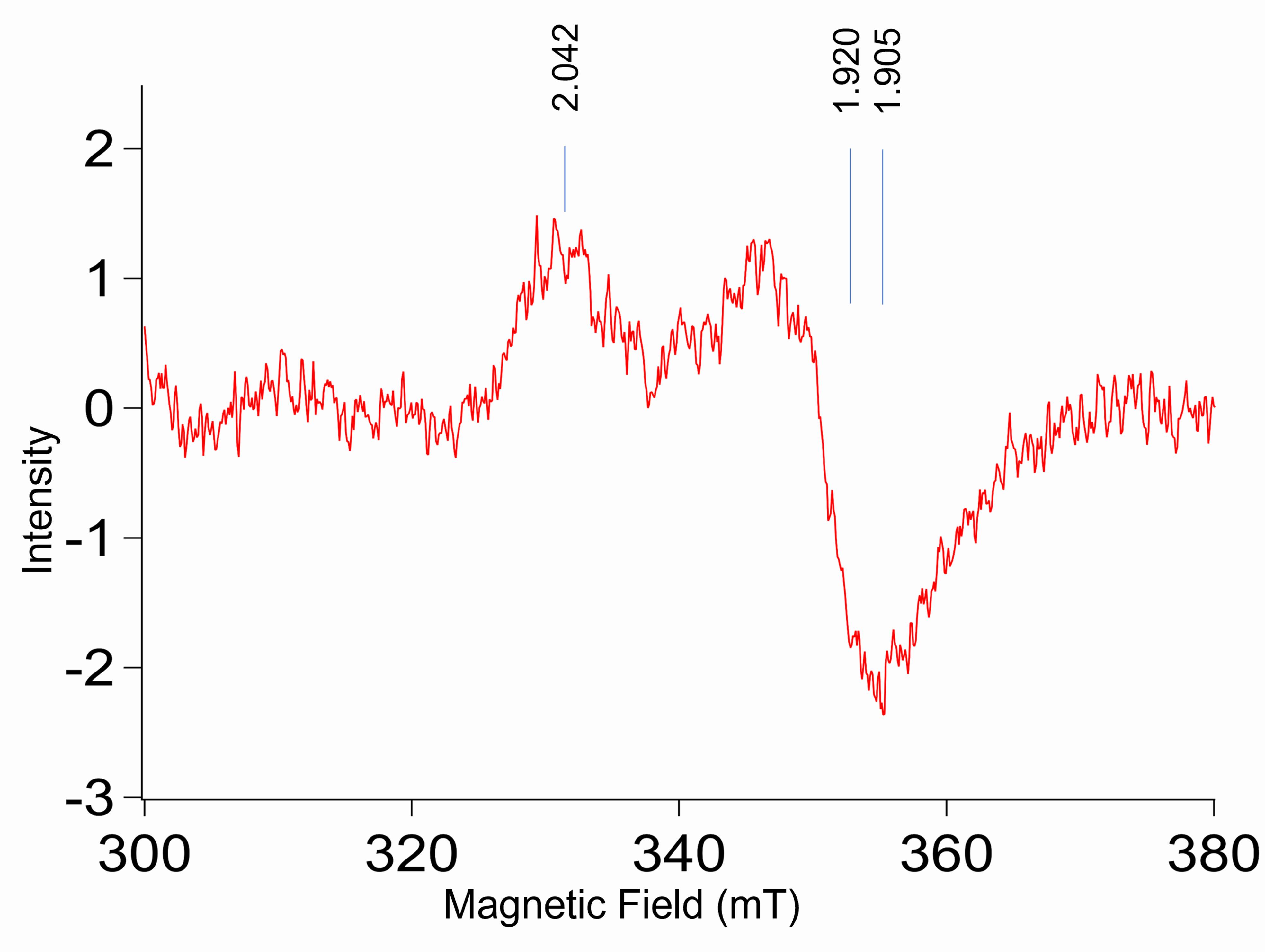
Figure 3. EPR spectra of CCIS. The EPR spectra of CCIS protein with g values indicating the presence of [4Fe-4S] cluster within the protein.To accurately determine the characteristic g-factor values of the [4Fe-4S]1+ signal, perform the EPR signal simulations using the EasySpin toolbox developed for Matlab (Stoll and Schweiger, 2006).
The quantitative yield of reduced [4Fe-4S]1+ clusters in the holo-peptide sample can be determined through spin counting analysis, where the integrated intensity of recorded [4Fe-4S]1+ is compared to the integrated intensity of the signal in an EPR-standard sample with a known number of spins (see Note 10). These analyses can be performed directly in the Xepr (Bruker) software.
ICP-AES to determine the amount of iron and sulfur in the CCIS protein
Subject 100 μl of 1 mg/ml of CCIS protein in buffer A to acid hydrolysis using 50% HNO3 in a clean glass test tube inside a water bath at 90°C.
Following overnight acid hydrolysis, dilute the sample using double distilled water.
The final volume of the sample is 3.7 ml, and the final concentration of HNO3 is approximately 2.5%.
Centrifuge the sample in 1.7 ml Eppendorf tubes at 4,427 × g for 5 min at 4°C.
Buffer A is treated in the same way as Steps G1-G4.
Make serial dilutions of the standard samples in the range of 0.1-5.0 ppm for iron and 0.5-100 ppm for sulfur, using 2.5% HNO3 (Figure 4).
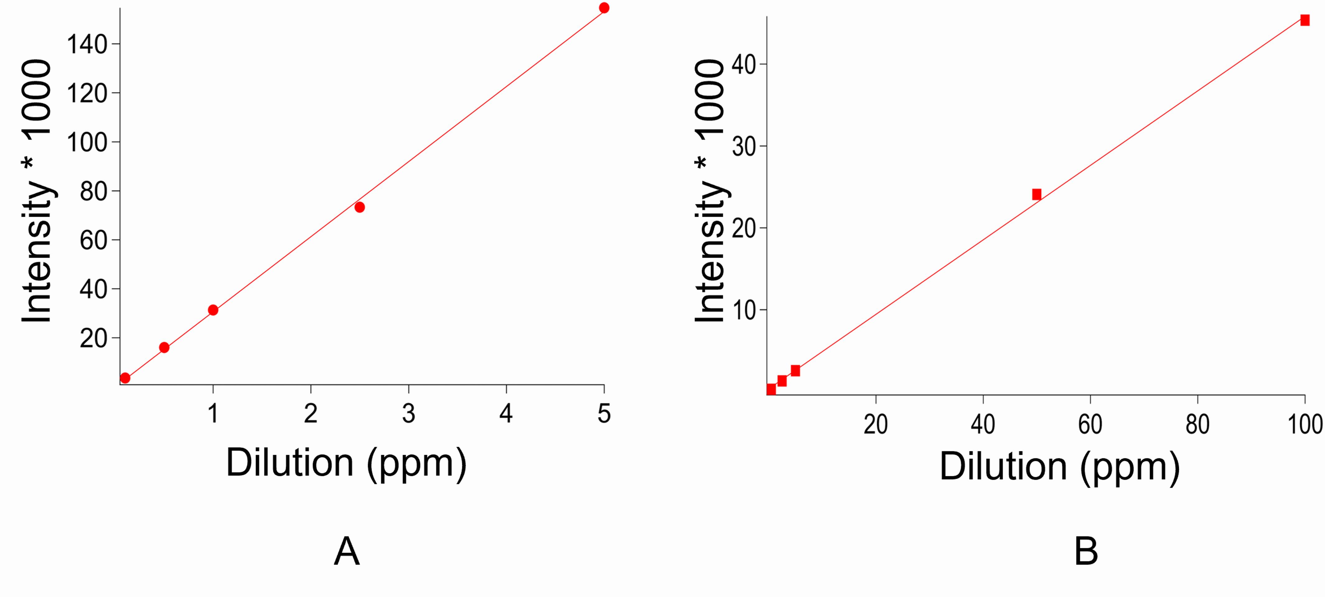
Figure 4. Standard curves from ICP-AES. A. The standard curve of Iron. B. The standard curve of Sulfur.Collect the data by selecting the wavelength 238.204 nm for quantifying iron content. Record for both standard, protein, and buffer individually.
Similarly, collect the data for quantifying sulfur by selecting 181.972 nm.
Subtract the corresponding blank values to determine the exact content of iron and sulfur individually.
Plot standard graphs for iron and sulfur individually and determine the values for the protein sample.
Data analysis
Data analysis for thermal denaturation of CCIS in the far UV region
Take the changes in the ellipticity values corresponding to 222 nm and plot against the temperature. To calculate the accurate melting temperature (Tm), use the equation described by Yadav and Ahmad (2000) or refer to the following equation:
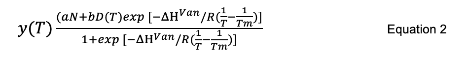
where,
a and b are two different temperature-independent constants,
N and D correspond to native and denatured states of the protein,
ΔHVan is the change in enthalpy,
R = 1.9872 × 10⁻³ kcal K−1 mol−1,
T is the temperature in Kelvin.
Open the data file (Excel file) in Igor Pro software.
Select the appropriate columns and plot graph; represent the data only in dots (do not plot line).
Under the ‘Analysis’ tab, select ‘Curve Fitting’ and then ‘New fit function.’
Give a name to the program under ‘fit function name.’
Under ‘Fit Coefficients’ tab, type “aD, bD, aN, bN, Tm, Hm.”
Under ‘Independent Variables,’ type ‘t”.
Compile the following code under ‘Fit expression’.
variable yN, yD, KD, R = 1.987e-3, Tk = t + 273.
yN = aN + bN × Tk
yD = (aD + bD × Tk)
KD = exp[-(Hm/R) × (1/Tk-1/Tm)]
f(t) = (yN + yD × KD)/(1+KD)
After compiling the code above, press ‘Test compile’ (see Note 11).
Save the fut function file by pressing ‘Save fit function now.’
Perform the nonlinear regression by selecting the above fit function and determine the Tm in Kelvin (see Note 12).
Data analysis for thermal denaturation of [4Fe-4S] cluster within holo-CCIS in the visible region
Take the changes in the ellipticity values corresponding to 400 nm and plot against the temperature. To calculate the accurate melting temperature (Tm), use equation 1 described in the supplementary data by Jagilinki et al. (2020) or refer to the following equation:
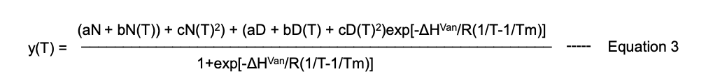
where,
a, b, and c are three different temperature-independent constants. For the remaining constants and variables, refer to details mentioned above in Equation 2.
Open the data file (Excel file) in Igor Pro.
Select the appropriate columns and plot graph; represent the data only in dots (do not plot line).
Under the ‘Analysis’ tab, select ‘Curve Fitting’ and then ‘New fit function.’
Give a name to the program under ‘fit function name.’
Under ‘Fit Coefficients’ tab, type “aD, bD, cD, aN, bN, cN, Tm, Hm.”
Under ‘Independent Variables,’ type ‘t”.
Compile the following code under ‘Fit expression’.
variable yN, yD, KD, R = 1.987e-3, Tk = t + 273.
yN = aN + bN × Tk + cN × Tk2
yD = aD + bD × Tk + cD × Tk2
KD = exp[-(Hm/R) × (1/Tk-1/Tm)]
f(t) = (yN + yD × KD)/(1 + KD)
After compiling the code above, press ‘Test compile’ (see Note 11).
Save the fut function file by pressing ‘Save fit function now.’
Perform the nonlinear regression by selecting the above fit function and determine the Tm in Kelvin (see Note 12).
Notes
Based on the 410/280 ratios, the number of iron–sulfur clusters present within the proteins can be estimated. CCIS monomer has three tryptophans in its sequence, and it is a holo-trimer. Therefore, the holo-protein has nine tryptophans and one [4Fe-4S] cluster, and the 410/280 ratio is expected to be low, approximately 0.2 in this case (Figure 1B). However, if the holo-CCIS was a dimer (6 W) or a monomer (3 W), the 410/280 ratio would be higher. A [4Fe-4S] protein with no tryptophan would have a significantly higher 410/280 ratio.
CD is highly sensitive to salts and buffer concentrations. Salt concentrations should typically be 50 mM or below.
In certain cases, metal binding stabilizes the secondary structure of the target protein; for example, CCIS has different CD spectra for the holo and apo forms.
For higher resolution spectra, scan at lower speeds up to 5 to 10 nm/s.
In most cases, there will be added thermal stability to the secondary structure of the holo-protein compared to apo-protein.
The entire experiment must be performed with the airtight lid on the cuvette to maintain the anaerobic nature of the holo-protein.
Longer incubation times are required because of the 1 cm path cuvette, which typically needs more time to achieve homogeneous temperature of the sample present in the cuvette.
The Na2S2O4 solution should be prepared freshly.
If the concentration of the protein is less than 200 µM, concentrate the protein using 10 kDa cut-off Centricon® at 4,000 rpm and 4°C under anaerobic conditions.
A small CuSO4·5H2O crystal with known weight can be used as an EPR spin-counting standard.
The code should not prompt any errors; otherwise, verify the code from the start.
To calculate the Tm in °C, subtract the Tm (in Kelvin) with 273.
Recipes
1 M Sodium dithionite (Na2S2O4)
Dissolve 0.174 mg of Na2S2O4 in 1 ml of double distilled water (see Note 8).
Buffer A
50 mM Tris-HCl pH 8.0
200 mM NaCl
Buffer B
10 mM Tris-HCl pH 8.0
40 mM NaCl
Buffer C
50 mM Tris-HCl pH 8.0
200 mM NaCl
15% Glycerol
Acknowledgments
D.N. acknowledges financial support from the Israel Science Foundation petroleum alternatives to transportation grant (GA 2185/17). D.N. and V.N. acknowledge the European Research Council (ERC) consolidator grant (GA615217). D.N., V.N., A.M.T., and B.P.J. were further supported by the NASA Astrobiology Institute Grant 80NSSC18M0093. The protocols described in this paper were adapted from various research articles characterizing iron-sulfur proteins published over five decades.
Competing interests
The authors declare no competing interests.
References
- Bertini, I., Ciurli, S. and Luchinat, C. (1995). The electronic structure of FeS centers in proteins and models a contribution to the understanding of their electron transfer properties. In: Iron-Sulfur Proteins Perovskites. Structure and Bonding, vol 83, pp 1-53. Springer, Berlin, Heidelberg.
- Freibert, S. A., Weiler, B. D., Bill, E., Pierik, A. J., Muhlenhoff, U. and Lill, R. (2018). Biochemical Reconstitution and Spectroscopic Analysis of Iron-Sulfur Proteins. Methods Enzymol 599: 197-226.
- Grzyb, J., Xu, F., Weiner, L., Reijerse, E. J., Lubitz, W., Nanda, V. and Noy, D. (2010). De novo design of a non-natural fold for an iron-sulfur protein: alpha-helical coiled-coil with a four-iron four-sulfur cluster binding site in its central core. Biochim Biophys Acta 1797(3): 406-413.
- Stoll, S. and Schweiger, A. (2006). EasySpin, a comprehensive software package for spectral simulation and analysis in EPR. J Magn Reson 178(1): 42-55.
- Beinert, H. (2000). Iron-sulfur proteins: ancient structures, still full of surprises. J Biol Inorg Chem 5(1): 2-15.
- Beinert, H. and Kiley, P. J. (1999). Fe-S proteins in sensing and regulatory functions. Curr Opin Chem Biol 3(2): 152-157.
- Brzoska, K., Meczynska, S. and Kruszewski, M. (2006). Iron-sulfur cluster proteins: electron transfer and beyond. Acta Biochim Pol 53(4): 685-691.
- Camprubi, E., Jordan, S. F., Vasiliadou, R. and Lane, N. (2017). Iron catalysis at the origin of life. IUBMB Life69(6): 373-381.
- Cordes, M. and Giese, B. (2009). Electron transfer in peptides and proteins. Chem Soc Rev 38(4): 892-901.
- Einsle, O. (2014). Nitrogenase FeMo cofactor: an atomic structure in three simple steps. J Biol Inorg Chem 19(6): 737-745.
- Flint, D. H. and Allen, R. M. (1996). Iron-Sulfur Proteins with Nonredox Functions. Chem Rev 96(7): 2315-2334.
- Fontecave, M. (2006). Iron-sulfur clusters: ever-expanding roles. Nat Chem Biol 2(4): 171-174.
- Gnandt, E., Dorner, K., Strampraad, M. F. J., de Vries, S. and Friedrich, T. (2016). The multitude of iron-sulfur clusters in respiratory complex I. Biochim Biophys Acta 1857(8): 1068-1072.
- Imlay, J. A. (2006). Iron-sulphur clusters and the problem with oxygen. Mol Microbiol 59(4): 1073-1082.
- Jagilinki, B. P., Ilic, S., Trncik, C., Tyryshkin, A. M., Pike, D. H., Lubitz, W., Bill, E., Einsle, O., Birrell, J. A., Akabayov, B., Noy, D. and Nanda, V. (2020). In Vivo Biogenesis of a De Novo Designed Iron-Sulfur Protein. ACS Synth Biol 9(12): 3400-3407.
- Johnson, D. C., Dean, D. R., Smith, A. D. and Johnson, M. K. (2005). Structure, function, and formation of biological iron-sulfur clusters. Annu Rev Biochem 74: 247-281.
- Kyritsis, P., Hatzfeld, O. M., Link, T. A. and Moulis, J. M. (1998). The two [4Fe-4S] clusters in Chromatium vinosum ferredoxin have largely different reduction potentials. Structural origin and functional consequences. J Biol Chem 273(25): 15404-15411.
- Liu, J., Chakraborty, S., Hosseinzadeh, P., Yu, Y., Tian, S., Petrik, I., Bhagi, A. and Lu, Y. (2014). Metalloproteins containing cytochrome, iron-sulfur, or copper redox centers. Chem Rev 114(8): 4366-4469.
- Lubitz, W., Chrysina, M. and Cox, N. (2019). Water oxidation in photosystem II. Photosynth Res 142(1): 105-125.
- Shaw, W. J., Helm, M. L. and DuBois, D. L. (2013). A modular, energy-based approach to the development of nickel containing molecular electrocatalysts for hydrogen production and oxidation. Biochim Biophys Acta 1827(8-9): 1123-1139.
- Wagner, T., Ermler, U. and Shima, S. (2016). The methanogenic CO2 reducing-and-fixing enzyme is bifunctional and contains 46 [4Fe-4S] clusters. Science 354(6308): 114-117.
- Yadav, S. and Ahmad, F. (2000). A new method for the determination of stability parameters of proteins from their heat-induced denaturation curves. Anal Biochem 283(2): 207-213.
Article Information
Copyright
© 2021 The Authors; exclusive licensee Bio-protocol LLC.
How to cite
Jagilinki, B. P., Paluy, I., Tyryshkin, A. M., Nanda, V. and Noy, D. (2021). Biophysical Characterization of Iron-Sulfur Proteins. Bio-protocol 11(20): e4202. DOI: 10.21769/BioProtoc.4202.
Category
Biophysics > EPR spectroscopy
Biochemistry > Protein > Activity
Do you have any questions about this protocol?
Post your question to gather feedback from the community. We will also invite the authors of this article to respond.