Pectin Nanostructure Visualization by Atomic Force Microscopy

Materials and Reagents

1. Tri-distilled butanol (VWR International, catalog number: 20810.323 )
   
2. Pectin fractions from cell wall extracts
   Notes:
   
   1. Cell wall extraction protocol is described in Posé et al. (2013).
      
   2. Pectin fractions from cell wall material are obtained by sequential extractions with CDTA buffer followed by sodium carbonate buffer, to solubilize a cell wall fraction enriched in ionically and covalently bound pectins respectively, as described in Posé et al. (2013) (see Recipes).
      
   3. Both pectin fractions (i.e., one extracted with CDTA and the other with sodium carbonate) were extensively dialyzed and stored until required at -20 ºC as aqueous solutions. Important: in order to prevent possible aggregation, any freeze-drying step must be avoided. It is recommended to aliquot the samples to avoid freeze-thawed successive cycles.
3. Ammonium bicarbonate (FLUKA, catalog number: 09830 )
   Note: Currently, it is “Sigma-Aldrich, catalog number: 09830”.
   
4. Trans-1,2-diaminocyclohexane-N,N,N'N'-tetra-acetic acid monohydrate (Sigma-Aldrich, catalog number: D 319945 )
   
5. Sodium carbonate (Sigma-Aldrich, catalog number: S2127 )
   
6. NaBH₄ (Sigma-Aldrich, catalog number: D 452882 )
   
7. 10 mM ammonium bicarbonate buffer (pH 8) (see Recipes)
   
8. CDTA buffer (see Recipes)
   
9. Sodium carbonate buffer (see Recipes)
   

Equipment

1. Acoustic-isolated and temperature-controlled room (Figure 1A-1)
   
2. Low-power light microscope, equipped with a television camera, was used to roughly position the AFM probe onto the top of the sample (Figure 1A-2)
   
3. Atomic Force Microscope (East Coast Scientific Limited, Cambridge, UK) (Figure 1A-3; Figure 2A). Any AFM of suitable resolution can be used, although the details of the software and liquid cell will vary
   
4. Anti-vibration table under the AFM microscope (Figure 1A-4)
   
5. Photodiode amplifier (Figure 1A-5)
   
6. Oscilloscope (Figure 1A-6; Figure 3)
   
7. Digital control system composed by computer, DAC (digital-to-analog converter) box, laser driver and high voltage amplifier. (for more details see Morris et al., 2010) (Figure 1A-7)
   
8. PYREX^® Culture Tubes with Rubber Liner Screw Caps (Thomas Scientific, catalog number: 9212C21 ) and Teflon-lined caps
   Note: The screw-capped glass tubes were acid washed using a 1% hydrochloric acid solution overnight then rinsed with water.
   
9. Sheets of mica (Elektron Technology, Agar Scientific, model: G250 ) cleaved with adhesive tape (3M, model: Magic Tape ) (Video 1)
   
10. Short tip variety AFM probe model contact cantilevers (Budget Sensors SiNi, Bulgaria)
    Note: The tip is mounted on the edge of a V-shaped cantilever, the typical geometry used for topographical imaging (Figure 1B).
    
11. Tip holder and open bucket liquid cell (Figure 1C; Vdeo 2)
    
12. Basic equipment: pipettes, vortex, sonicator bath, heating block
    
    
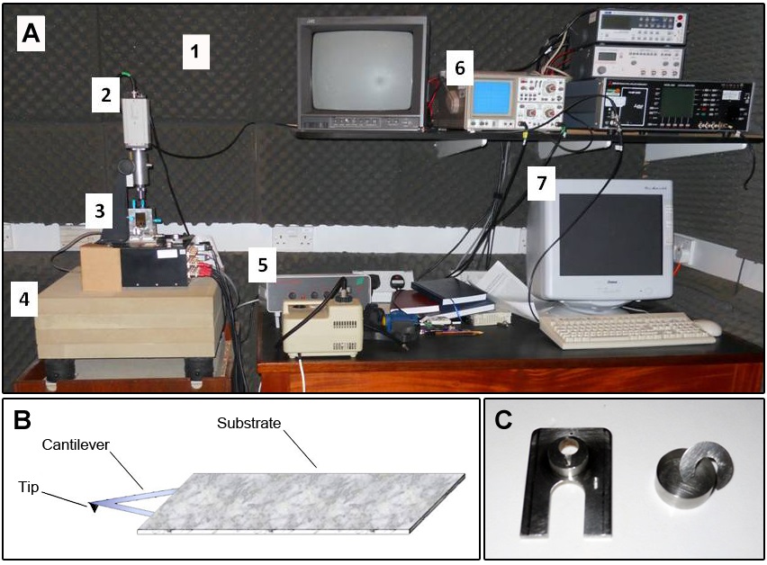
    Figure 1. Atomic force microscopy (AFM) equipment. A. Photograph including an overview of AFM room set-up. The numeric labels are in accordance with the equipment list description. B. Scheme of a sharp tip located at the free end of a cantilever. C. Detail of tip holder (left) and liquid cell (right).
    

Software

1. AFM software supplied with the instrument (SPM 6.01, ECS, Cambridge, UK)
   
2. For the length measurements, images were converted to TIFF files using Paint Shop Pro v5.00 software (http://web.archive.org/web/19980514080113/http://jasc.com/)
   
3. Image contrast and 3D effects were optimized using Gwyddion software v2.32
   
4. AFM images were analyzed off-line using Image J v1.43u software (http://imagej.nih.gov/ij/index.html)
   
5. Gwyddion is free and open source software, covered by GNU (General Public License) (http://gwyddion.net/)
   

Procedure

First preparative step, at the acoustic-isolated and temperature-controlled room, is to turn on air conditioning and all the AFM equipment (PC, monitor, amplifiers…) to avoid background noise during AFM scanning. In the meantime, you can prepare your samples as described next.

1. Sample preparation
   
   1. Dilute pectin solution (pectin fractions obtained with CDTA and sodium carbonate buffer) in pure water to 1 mg/ml and heat at 80 °C for 30 min.
      
   2. Make a serial dilution in 10 mM ammonium bicarbonate^* to a final concentration of 1-5 μg/ml. The required volume depends on the initial concentration of the sample taking into account that it would only 3 μl would be required for AFM. Dilutions must be prepared freshly just before used. A sublimable buffer is used to prevent deposition of buffer crystals on the mica substrate, because they don´t leave residual salt crystals when evaporates.
      
   3. Warm up the sample at 80 °C for 20 min and immerse in ultrasonic bath^* for 10 min. ^*(only for sodium carbonate fraction; for CDTA fraction both dilution steps are done with pure water and the ultrasonic step is omitted). This step promotes disaggregation of cell wall networks to enable visualization of isolated chains.
      
   4. Reshape the mica to the final size, which will fit the liquid cell, and cleave the sheet by inserting a sharp tip on the corner or peeling off the outer sheets with adhesive tape (Video 1). Always use tweezers to manipulate mica and keep them covered to protect from dust.
      
      
      
      Video 1. How to cleave the mica
      
      
   5. Pipette out 3 μl of the CDTA or sodium carbonate pectin sample onto freshly cleaved mica and dry over a heating stage at 37-40 °C for 20 min, in order to promote even spreading, to reduce molecular aggregation and to sublime off the buffer before imaging.
      Note: Incubation times, temperature and dilutions must be optimized for different polymers, always keeping in mind that those parameters must be consistent amongst samples that will be compared with each other.
   
   
2. Atomic force microscopy
   
   6. Insert the sample into the liquid cell of the microscope (Figure 1C) and inject 300 μl of tri-distilled butanol into the cell, halfway of the sample approach sequence. The use of butanol as an imaging solvent has a double purpose; it eliminates capillary condensation but also is a precipitant for polysaccharides, so prevents desorbing of the polysaccharide during imaging.
      
   7. AFM tip probe is mounted on the tip holder (Figure 1B; Video 2), inserted into the microscope (Figure 1A-3) and roughly positioned onto the top of the sample using a low-power microscope equipped with a television camera (Figure 1A-2). The sharpness of the tip determines the resolving power of the instrument, so must be carefully manipulated as it can be blunted or contaminated with polysaccharide if driven into direct contact with the substrate.
      
      
      
      Video 2. How to mount sample on open bucket cell
      
      
   8. Align laser and detector beams onto the tip using the four-quadrant photodiode and amplifier (Figure 2). In this case the tips used have a resonant frequency and force constant of 13 KHz and 0.4 N/m, respectively.
      
      1. Align the laser beam: The laser alignment knobs (represented by red arrows in Figure 2B) are used to move the laser in the X and Y directions until the laser spot is positioned on the end of the cantilever (Figure 2D). An optical microscope is used to visualise the laser spot and cantilever to check if the laser is aligned (Figure 2C-D)
         
      2. Align photodetector to the laser beam: Once the laser is aligned onto the cantilever, two different screws are used (represented with yellow arrows in Figure 2B) to position the photodiode so that it captures the reflected laser spot. Once it detects the reflected laser beam the photodiode must be finely adjusted to position the laser spot to a perfectly central position on the 4 quadrants of the photodiode. If the laser is not properly positioned on the cantilever, it will be impossible to detect the reflected spot with the photodiode. The total voltage generated by the photodetector is shown in the electronic-combined box (Figure 2F). The level of cantilever deflection is shown in Figure 2E. This indicates the voltage difference between the top and bottom segments of the photodetector. For the contact mode, the deflection signal of the photodetector has to be close to zero.
         
         
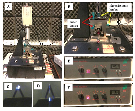
         Figure 2. Atomic force microscope basic set-up. A. Atomic force microscope. B. AFM knobs to align the laser beam and photodetector. C. Probe with laser aligned. D. Probe with laser not aligned correctly. E. Photodetector amplifier with axis data. F. Photodetector amplifier with SUM data.
      
      
   9. Approach the sample to the tip to subtly position the tip onto the sample surface. This step must be done carefully to avoid hitting the tip onto the sample, which will blunt or contaminate the tip and ruin the scanned image. This step is done with the support of an oscilloscope (Figure 3) that reproduces the vibration of the cantilever. When the tip is far from the sample, the vibration waves will be broad (Figure 3A) and when the tip closely approaches the surface the wave pattern will a make sudden change denoting that tip and sample are establishing contact (Figure 3B). Adjust the force to obtain a good resolution during the scanning. Increasingly in modern AFMs this approach step is automatic.
      
      
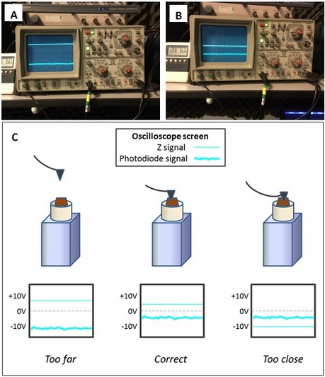
      Figure 3. Oscilloscope output signals when tip and sample are at a far (A) or in correct (B) position. C. Scheme of different tip positions on the sample and its oscilloscope output signal. (see how those lines behave during the approaching sequence in Video 3)
      
      
      
      Video 3. A general overview of AFM method
      
      
   10. Once everything is mounted and aligned, it is recommended to leave the sample and instruments 1 hour at 20 °C to equilibrate temperature and reduce background noise during scanning.
       
   11. The imaging is scanned at a scan speed of 2 Hz.
       
   12. AFM acquires data simultaneously from the movement of the feedback loop in the z-axis to keep a constant force during scanning (topographical mode image), and from the cantilever deflection (error signal image) with additional information about topography. Both topographical (Figure 4B) and error signal (Figure 4A) mode images are collected.
       Note: See Video 3 for a general overview of AFM method. Further information about alternative scanning modes and AFM in other biological samples are described in Morris et al. (2010).
   
   
3. AFM image analysis
   
   13. Height measurements. The heights of features are analyzed using the AFM software supplied with the instrument (SPM 6.01, ECS, Cambridge, UK), which fits a plane and re-normalizes the AFM images. Topographical data is crucial for distinguishing true branch points from overlapping chains, where the height is doubled, and these are easily visualized as they appear as bright points at the crossing points on the chain (Figure 4).
       
       
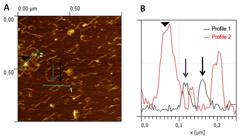
       Figure 4. AFM image analysis for true branch point verification. A. Representative image of CDTA pectins from ripe strawberry fruit obtained by AFM in contact mode. Branched pectin chains and micellar aggregates with emerging strands can be observed in the image. B. Height profiles, showing the heights in a true branch point (black arrow) of a polymer chain (profile 1) and micellar aggregates (profile 2) with emerging strands of same height than isolated chains (grey arrow) and higher height at the core area (arrowhead). Reprinted from Posé et al. (2015) with permission from Elsevier.
       
       
   14. Length measurements. The images are converted to TIFF files using Paint Shop Pro v 5.00 software. Image contrast and 3D layouts are performed by Gwyddion v 2.32 software. Then, the images are analyzed offline using ImageJ v1.43u software by plotting the strands with the freehand tool of the software. To determine the chain lengths only isolated chains, defined as individual strands that are not entangled with other strands, that are long enough to be exactly visualized, and which lay entirely within the scanned area are measured. The total length of the chain, including branches if any, is defined as the contour length.
       
       
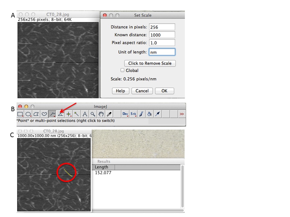
       Figure 5. ImageJ workflow. A. First set the scale of your scan size (e.g., 256 pixels correspond to 1,000 nm). B. Chose freehand tool and draw the chains. C. Click CTRL+M and a new data window will prompt with the data measurements.
       
       
   15. Data analysis for length measurement.
       The contour length can be represented by histograms with the frequency of occurrence of particular lengths plot against the molecular length (Figure 6). Because polymers are mixtures of molecules of different molecular weight, they are naturally polydisperse, and their characterization is not well described with a single average. Instead, AFM data is characterized measuring the number-average () and the weight-average () contour length, as well as the ratio of the two average polymer lengths (), called polydispersity index (PDI). () is an arithmetic average (a), () is a weight average (b) that compensates the bias of a higher count of small chains over large ones (because is more likely to encounter small chains fully visualized in the scan area), and PDI a parameter to define the breadth of the distribution curve (Posé et al., 2012). This PDI index would be unity for a perfectly monodisperse polymer, so the higher the value the more disperse the polymer.
       
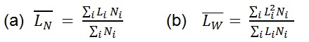
       An example of the intermediate calculations is included in table 1. Briefly, once contour length data is collected, interval Range should be defined (e.g., 0-25; 25-50; 50-100…), as well as the Frequency for each interval and its Mark Class (average interval range value). Then:
       Total (N) = Total number of data
       SUM1 = ∑ Mark Class x Frequency
       SUM2 = ∑ Mark Class x SUM1 
         = SUM1 / N
         = SUM2 / SUM1
       PDI =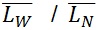
       
       Table 1. AFM contour length analysis and intermediate calculations to obtain L_N, L_W and PDI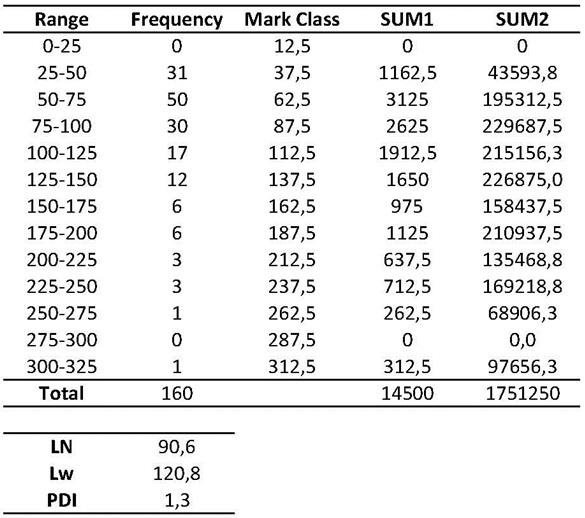
       
       
       
   16. Branching pattern. When true branch points are present, the number of branching points per isolated strand and their lengths can be measured. When equivalent dilutions are employed, the number of branched chains per scanned area can be used to define the percentage of branched polymers within a sample. Differences in the branching of the polymer chains, presence/absence of side chains and the number of side chains per backbone, are analyzed by a Chi-square test.
       
   17. Statistical distribution. Usually the frequency is a right skewed distribution which does not fit a normal distribution and median (ME) is the statistical parameter to analyze samples with Kruskal–Wallis test (Posé et al., 2012). Further statistical analysis of right skewed distributions data (Figure 6A-B) can be done by fitting a Log normal distribution to the data (Posé et al., 2012). Thus, if original data (L) is transformed by natural logarithm a normal distribution is obtained, and the data can be compared by analysis of variance (ANOVA). Another useful option for sample analysis is the cumulative frequency curves generated by the Log normal function (Figure 6C).
       
       
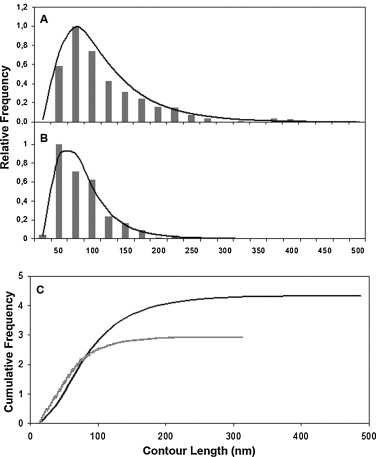
       Figure 6. Contour length distribution from CDTA (A) and sodium carbonate (B) soluble polymers. Bars represent observed data whilst the curved lines represent Log normal approximations. C. Cumulative frequencies for CDTA (black line) and Na₂CO₃ (grey line) pectic fractions by Log normal function normalized to the maximum peak obtained in each profile. N = 379 and 372 for CDTA and Na₂CO₃ samples, respectively. Reprinted from Posé et al. (2012) with permission from Elsevier.
       
       Note: It is recommended to analyze at least three dozen AFM images for each condition, with a minimum of 100 independent measurements of isolated chains from different images, to obtain a representative sample. Once everything is optimized, an AFM image is done every 5 min. See Video 3 for a general overview of AFM method.

Recipes

1. 10 mM ammonium bicarbonate buffer (pH 8)
   Sterilized Millipore water filter is used.
   Either formic acid (HCOOH) or ammonium hydroxide (NH₄OH) are recommended to adjust ammonium bicarbonate pH 8 buffer.
   
2. CDTA buffer
   0.05 M trans-1,2-diaminocyclohexane-N,N,N'N'-tetraacetic acid in 0.05 M sodium acetate buffer (pH 6; adjust with Potassium Hydroxide KOH)
   Stored at RT
   
3. Sodium carbonate buffer
   0.1 M sodium carbonate containing 0.1% NaBH₄ freshly added
   Stored at RT but always add NaBH₄ just before use
   Caution: NaBH₄ is toxic, corrosive and dangerous when wet. Inhalation and contact with skin should be prevented.
   

Acknowledgments

Figure 4 is reprinted from Posé et al. (2015). Figure 6 is reprinted from Posé et al. (2012) with permission from Elsevier. This work was funded by the Ministerio de Educación y Ciencia of Spain and Feder EU Funds (grant reference: AGL2011-24814). The research at IFR was supported through the BBSRC core grant to the Institute.

References

1. Liu, D. and Cheng, F. (2011). Advances in research on structural characterisation of agricultural products using atomic force microscopy. J Sci Food Agric 91(5): 783-788.
   
2. Morris, V. J., Kirby, A. R. and Gunning, A. P. (2010). Atomic Force Microscopy for Biologists. 2nd ed. Imperial College Press ISBN-10: 184816467X.
   
3. Paniagua, C., Pose, S., Morris, V. J., Kirby, A. R., Quesada, M. A. and Mercado, J. A. (2014). Fruit softening and pectin disassembly: an overview of nanostructural pectin modifications assessed by atomic force microscopy. Ann Bot 114(6): 1375-1383.
   
4. Posé, S., Kirby, A. R., Mercado, J. A., Morris, V. J. and Quesada, M. A. (2012). Structural characterization of cell wall pectin fractions in ripe strawberry fruits using AFM. Carbohyd Polym 88: 882-890.
   
5. Posé, S., Kirby, A. R., Paniagua, C., Waldron, K. W., Morris, V. J., Quesada, M. A. and Mercado, J. A. (2015). The nanostructural characterization of strawberry pectins in pectate lyase or polygalacturonase silenced fruits elucidates their role in softening. Carbohyd Polym 132: 134-145.
   
6. Posé, S., Paniagua, C., Cifuentes, M., Blanco-Portales, R., Quesada, M. A. and Mercado, J. A. (2013). Insights into the effects of polygalacturonase FaPG1 gene silencing on pectin matrix disassembly, enhanced tissue integrity, and firmness in ripe strawberry fruits. J Exp Bot 64(12): 3803-3815.
   
7. Zdunek, A., Koziol, A., Pieczywek, P. M. and Cybulska, J. (2014). Evaluation of the nanostructure of pectin, hemicellulose and cellulose in the cell walls of pears of different texture and firmness. Food Bio Tech 7 (12): 3525-3535.