
- Home
- Protocols

-

Association between the Wuhan city travel ban and the arrival time of COVID-19 in other cities
Last updated date: Feb 1, 2021 Views: 1091 Forks: 0
Here we quantify the association between the Wuhan travel shut- down (23 January 2020) and COVID-19 spread.
rm(list = ls())
library(readxl)
library(car)
## Loading required package: carData
library(lmtest)
## Loading requiredpackage: zoo ##
## Attaching package: 1zoo1
## The following objects are maskedfrom 1package:base1: ##
## as.Date,as.Date.numeric
library(sandwich)
library(fitdistrplus)
## Loadingrequired package: MASS
## Loading requiredpackage: survival
## Loading requiredpackage: npsurv
## Loadingrequired package: lsei
library(R330)
## Loading requiredpackage: s20x
##
## Attaching package: 1s20x1
## The following object is masked from 1package:car1:
##
## levene.test
## Loading requiredpackage: leaps ##Loading required package: rgl
## Loading required package: lattice
infected=read_xlsx("./Travel_ban_model.xlsx",sheet="1")
Processing the data
infectedW=infected[infected$arrivalday>=2,]
infectedW$Totalflow=infectedW$Train2018+infectedW$Road2018+infectedW$Air2018+1
Regression analysis
The association between distance, human movement, interventions and timing of COVID-19 spread was assessed by a linear regression.
fit <- lm(arrivalday~lat+lon+log10(Pop2018)+log10(Distance)+ log10(Train2018+1)+ log10(Air2018+1)+ log10(Road2018+1)+log10(Totalflow)+aftershutdown,
data=infectedW)
lm.step<-step(fit)
## Start: AIC=113.73
## arrivalday ~ lat + lon + log10(Pop2018) + log10(Distance) + log10(Train2018 +
## 1) + log10(Air2018 + 1) + log10(Road2018 + 1) + log10(Totalflow) +
## aftershutdown
##
| ## | Df Sum of Sq | RSS | AIC | ||
| ## | - log10(Train2018 + 1) | 1 | 0.26 | 374.03 | 111.91 |
| ## | - log10(Air2018 + 1) | 1 | 0.98 | 374.75 | 112.41 |
| ## | - log10(Road2018 + 1) | 1 | 1.12 | 374.89 | 112.51 |
| ## | - log10(Totalflow) | 1 | 2.37 | 376.14 | 113.38 |
| ## | <none> | 373.77 | 113.73 | ||
| ## | - log10(Distance) | 1 | 3.54 | 377.30 | 114.19 |
| ## | - lat | 1 | 3.80 | 377.57 | 114.37 |
| ## | - log10(Pop2018) | 1 | 8.37 | 382.14 | 117.51 |
| ## | - lon | 1 | 8.47 | 382.24 | 117.58 |
| ## | - aftershutdown | 1 | 331.09 | 704.86 | 277.30 |
| ## | |||||
## Step: AIC=111.91
## arrivalday ~ lat + lon + log10(Pop2018) + log10(Distance) + log10(Air2018 +
## 1) + log10(Road2018 + 1) + log10(Totalflow) + aftershutdown
##
| ## | Df | Sum ofSq | RSS | AIC | |
| ## | - log10(Road2018 + 1) | 1 | 1.04 | 375.07 | 110.63 |
| ## | - log10(Air2018 + 1) | 1 | 1.79 | 375.82 | 111.16 |
| ## | <none> | 374.03 | 111.91 | ||
| ## | - lat | 1 | 3.61 | 377.64 | 112.42 |
| ## | - log10(Distance) | 1 | 3.81 | 377.84 | 112.56 |
| ## | - log10(Totalflow) | 1 | 3.90 | 377.93 | 112.62 |
| ## | - lon | 1 | 8.22 | 382.25 | 115.58 |
| ## | - log10(Pop2018) | 1 | 9.12 | 383.14 | 116.19 |
| ## | - aftershutdown | 1 | 333.03 | 707.05 | 276.11 |
##
## Step: AIC=110.63
## arrivalday ~ lat + lon + log10(Pop2018) + log10(Distance) + log10(Air2018 +
## 1) + log10(Totalflow) + aftershutdown
##
| ## | Df | Sum of Sq | RSS | AIC | |
| ## | - log10(Air2018 + 1) | 1 | 1.73 | 376.80 | 109.83 |
| ## | - log10(Distance) | 1 | 2.79 | 377.85 | 110.57 |
| ## | - log10(Totalflow) | 1 | 2.88 | 377.95 | 110.63 |
| ## | <none> | 375.07 | 110.63 | ||
| ## | - lat | 1 | 4.94 | 380.01 | 112.05 |
| ## | - lon | 1 | 8.89 | 383.95 | 114.74 |
| ## | - log10(Pop2018) | 1 | 11.60 | 386.66 | 116.58 |
| ## | - aftershutdown | 1 | 333.21 | 708.27 | 274.56 |
##
## Step: AIC=109.83
## arrivalday ~ lat + lon + log10(Pop2018) + log10(Distance) + log10(Totalflow) +
## aftershutdown
##
| ## | Df | Sum of Sq | RSS | AIC | |
| ## | - log10(Distance) | 1 | 1.07 | 377.87 | 108.58 |
| ## | <none> | ||||
| ## | - log10(Totalflow) | 1 | 5.90 | 382.69 | 111.89 |
| ## | - lat | 1 | 6.72 | 383.51 | 112.45 |
| ## | - lon | 1 | 9.50 | 386.30 | 114.33 |
| ## | - log10(Pop2018) | 1 | 12.85 | 389.64 | 116.58 |
| ## | - aftershutdown | 1 | 346.90 | 723.70 | 278.18 |
##
## Step: AIC=108.57
## arrivalday ~ lat + lon + log10(Pop2018) + log10(Totalflow) +
## aftershutdown
##
| ## | Df | Sum of Sq | RSS | AIC | |
| ## | <none> | 377.87 | 108.58 | ||
| ## | - log10(Totalflow) | 1 | 7.63 | 385.50 | 111.79 |
| ## | - lat | 1 | 9.98 | 387.84 | 113.38 |
| ## | - lon | 1 | 12.11 | 389.98 | 114.81 |
| ## | - log10(Pop2018) | 1 | 15.75 | 393.61 | 117.23 |
| ## | - aftershutdown | 1 | 351.56 | 729.42 | 278.24 |
Selection model
Among five possible regression models examined, the model judged best by the Akaike Information Criterion.
step.model <- stepAIC(fit, direction = "backward", trace = FALSE)
summary(step.model)
##
## Call:
## lm(formula = arrivalday ~ lat + lon + log10(Pop2018) + log10(Totalflow) +
## aftershutdown, data = infectedW)
##
## Residuals:
## Min 1Q Median 3Q Max
## -4.5232 -0.8999 0.0366 0.8347 2.7326
##
## Coefficients:
| ## | Estimate Std. | Error | t value | Pr(>|t|) | ||
| ## | (Intercept) | 25.95350 | 1.28100 | 20.260 | < 2e-16 | *** |
| ## | lat | 0.03235 | 0.01247 | 2.595 | 0.01001 | * |
| ## | lon | -0.03219 | 0.01126 | -2.859 | 0.00460 | ** |
| ## | log10(Pop2018) | -0.69636 | 0.21361 | -3.260 | 0.00127 | ** |
| ## | log10(Totalflow) | -0.11786 | 0.05194 | -2.269 | 0.02409 | * |
| ## | aftershutdown | 2.91307 | 0.18913 | 15.403 | < 2e-16 | *** |
| ## | --- |
## Signif. codes: 0 1***10.001 1**1 0.01 1*1 0.051.1 0.1 1 1 1
##
## Residual standarderror: 1.217 on 255 degreesof freedom
## Multiple R-squared: 0.589, Adjusted R-squared: 0.581
## F-statistic: 73.1 on 5 and 255 DF, p-value: <2.2e-16
There appears to be five influential points.
influencePlot(step.model)
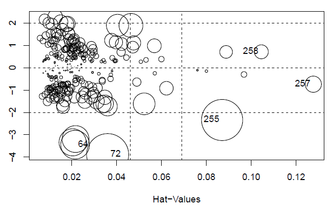
## StudRes Hat CookD
## 64 -3.4440481 0.02149690 0.041656769
## 72 -3.8878442 0.03598356 0.089102090
## 255-2.3402866 0.08700970 0.085492844
## 257-0.7385126 0.12764904 0.013324957
## 258 0.7114217 0.10448601 0.009861219
Removing the five influential points does not affect the conclusions.
step.model.1 <- lm(arrivalday~lat+lon+log10(Pop2018)+log10(Totalflow)+aftershutdown, data=infectedW[-c(64,72,255,257,258),])
summary(step.model.1)
##
## Call:
## lm(formula = arrivalday ~ lat + lon + log10(Pop2018) + log10(Totalflow) +
## aftershutdown, data = infectedW[-c(64, 72, 255, 257,258),
## ])
##
## Residuals:
## Min 1Q Median 3Q Max
## -4.0551 -0.8616 0.0285 0.7634 2.7182
##
## Coefficients:
| ## | Estimate Std. | Error | t value | Pr(>|t|) | |
| ## | (Intercept) | 26.41984 | 1.35511 | 19.496 < 2e-16 | *** |
| ## | lat | 0.03787 | 0.01267 | 2.989 0.003079 | ** |
| ## | lon | -0.03582 | 0.01246 | -2.874 0.004399 | ** |
| ## | log10(Pop2018) | -0.75115 | 0.20467 | -3.670 0.000296 | *** |
| ## | log10(Totalflow) | -0.12542 | 0.04919 | -2.550 0.011375 | * |
| ## | aftershutdown | 2.74963 | 0.18132 | 15.165 < 2e-16 | *** |
| ## | --- |
## Signif. codes: 0 1***1 0.0011**1 0.01 1*1 0.05 1.1 0.1 1 1 1
##
## Residual standarderror: 1.15 on 250 degreesof freedom
## Multiple R-squared: 0.5949, Adjusted R-squared: 0.5868
##F-statistic: 73.42 on 5 and 250 DF, p-value: <2.2e-16
There are still influential points.
influencePlot(step.model.1)
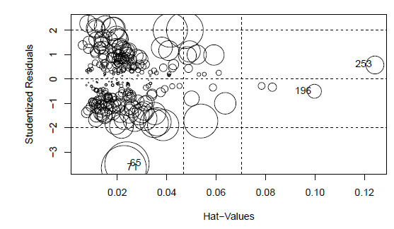
| ## StudRes | Hat | CookD |
## 65 -3.4840025 | 0.02393807 | 0.047499266 |
## 71 -3.6542347 | 0.02267970 | 0.049214740 |
## 196 -0.5048840 | 0.09978582 | 0.004723362 |
## 253 0.5730018 | 0.12425452 | 0.007785087 |
The Cook’s distances do not indicate presence of outliers. Here are a number of observations indicated as having large hat values. However, they are not too far away from they cutoff, and their hat values are quite
similar to each other. So it is hard to justigy removing only a subset of those points, but there are quite a few of them, so we leave them in the model.
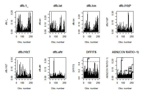
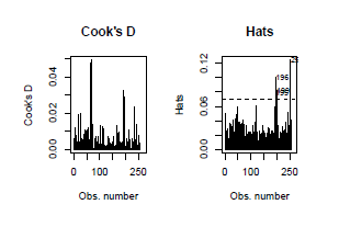
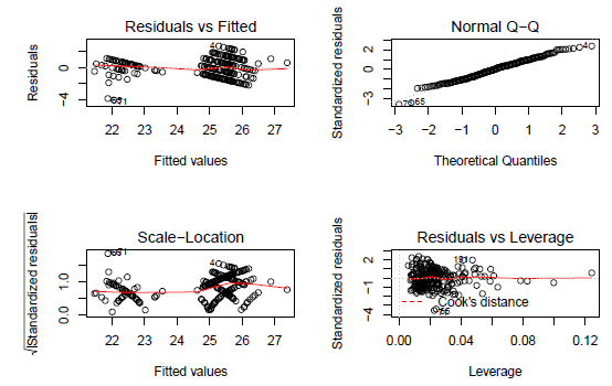
par(mfrow = c(2,4))
influenceplots(step.model.1)
We did not detect issuesregarding heteroscedasticity (studentized Breuch-Pagan test P=0.20)nor normality (Shapiro-Wilk test P=0.06).
lmtest::bptest(step.model.1)
##
## studentized Breusch-Pagan test
##
## data: step.model.1
## BP = 7.2846, df = 5, p-value = 0.2003
shapiro.test(step.model.1$residuals)
##
## Shapiro-Wilk normality test
##
## data: step.model.1$residuals
## W = 0.98961, p-value= 0.06359
The plot of studentised residuals does not indicate evident non-linearity in the residuals.
par(mfrow = c(2,2))
plot(step.model.1)
Diagnostics
Check for spatial correlation in the residuals
Here we performed additional checks to investigate whether there was spatial autocorrelation among the residuals, which could contribute to data dependency. If there were spatial autocorrelation in the residuals, then the pairwise residual differences of cities closer together would tend to be smaller than those of cities far apart. In other words, we would expect a high correlation between the pairwise differences in residuals and pairwise distances of cities. Such a correlation was not evident (r=0.03).
fit.res.dist.mat = as.matrix(dist(residuals(step.model, type = "pearson")))
gcs.dist.mat=as.matrix(dist(data.frame(infectedW$lon,infectedW$lat)))
cor.test(gcs.dist.mat,fit.res.dist.mat)
##
## Pearson1s product-moment correlation
##
## data: gcs.dist.mat and fit.res.dist.mat
## t = 8.5113, df = 68119,p-value < 2.2e-16
## alternative hypothesis: true correlation is not equalto 0
## 95 percent confidence interval:
## 0.025090330.04009330
## sample estimates:
## cor
## 0.03259365
Differential accessibility from Wuhan to other cities may contribute to data-dependence. Therefore, we examined the timing of peak inflow from Wuhan City and the arrival time of COVID-19 in each city. The result shows no evident correlation between them (r=-0.07, P=0.25).
cor.test(infectedW$peak_time2,infectedW$arrivalday)
##
## Pearson1s product-moment correlation
##
## data: infectedW$peak_time2 and infectedW$arrivalday
## t = -1.1663,df = 246, p-value = 0.2446
## alternative hypothesis: true correlation is not equalto 0
## 95 percent confidence interval:
## -0.19690241 0.05088306
## sample estimates:
## cor
## -0.07415409
In addition, we calculated the correlation between the residuals and peak time of Wuhan inflow during 11 to 23 January (15 days before Chinese New Year to the Wuhan shutdown). Again, we found no evident correlation (r=-0.08, P=0.20).
cor.test(step.model$residuals,infectedW$peak_time1)
##
## Pearson1s product-moment correlation
##
## data: step.model$residuals and infectedW$peak_time1
## t = -1.2948,df = 246, p-value = 0.1966
## alternative hypothesis: true correlation is not equalto 0
## 95 percent confidence interval:
## -0.2047447 0.0427291
## sample estimates:
## cor
##-0.08227597
- Liu, Y and Wu, C(2021). Association between the Wuhan city travel ban and the arrival time of COVID-19 in other cities. Bio-protocol Preprint. bio-protocol.org/prep802.
- Tian, H., Liu, Y., Li, Y., Wu, C., Chen, B., Kraemer, M. U. G., Li, B., Cai, J., Xu, B., Yang, Q., Wang, B., Yang, P., Cui, Y., Song, Y., Zheng, P., Wang, Q., Bjornstad, O. N., Yang, R., Grenfell, B. T., Pybus, O. G. and Dye, C.(2020). An investigation of transmission control measures during the first 50 days of the COVID-19 epidemic in China . Science 368(6491). DOI: 10.1126/science.abb6105
Do you have any questions about this protocol?
Post your question to gather feedback from the community. We will also invite the authors of this article to respond.