Electromagnetic simulation

Electromagnetic Simulation Instructions

The coil design can be modeled directly in the HFSS using the geometry/drawing tools or it can be imported from an external drafting software (e.g., AutoCAD)

A. To determine the inductance, Q factor and S₁₁
1. Import the coil geometry into the HFSS software.

1. Assign the material properties to the coil by selecting the HFSS material library.
2. Create an air sphere (radius 750 mm) and assign a radiation boundary.
3. Create a Lumped Port at the location of the capacitor in Figure 1A to assign the excitation with default port impedance values.
4. In the Analysis tab, select the solution frequency and assign a frequency sweep to obtain the electromagnetic properties as a function of frequency.
5. Validate the model (e.g., check all the simulation set up is correct) and run the simulation
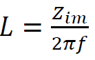
6. Create output variables for the inductance and Q factor as and 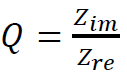where 𝑍_𝑟𝑒, 𝑍_𝑖𝑚, and 𝑓, are the real and imaginary parts of the port impedance 𝑍 and the frequency, respectively.
7. In the Results tab, plot the L and Q using the rectangular plot for the output variables.
8. Change the default port impedance in step 4 to the reactance calculated from the matching capacitor for the solution frequency.
9. Validate the model (e.g., check all the simulation set up is correct) and re-run the simulation
10. In the Results tab, plot the S₁₁ using the rectangular plot for the S-Parameters.

B. To determine the power transfer efficiency

1. Import both transmission and receiver coil geometry into the HFSS software.
2. Assign the material properties to the coils by selecting the HFSS material library.
3. Create an air sphere (radius 750 mm) and assign a radiation boundary.
4. Replace the Lumped Port from the previous step 4 for an RLC boundary condition (e.g., matching capacitor) in the receiver coil in Figure 1A(i)
5. To model the conditions of the real device, assign an RLC boundary (e.g., resistor) between the anode and cathode (Figure 1A) to account for the resistor (measured in the experiment), just like in the real device.
6. Create a Lumped Port for the transmission coil in Figure 1E to assign the excitation with default port impedance values.
7. Validate the model (e.g., check all the simulation set up is correct) and run the simulation.

8. Calculate the voltage difference ∆𝑉 between the two ends of the resistor added in step 5 using the Calculator Function. (further details on how to use the Calculator can be found in the HFSS Field Calculator Cookbook online).

9. Calculate the Power in the receiver coil load as .
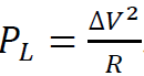10. Calculate the transfer efficiency as 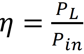 , where 𝑃 is the input power in the transmission antenna (in HFSS the default 𝑃_𝑖𝑛  is 1W, but this value can be changed depending on the application).

Category