Chromatin IP with reference exogenous genome

Abstract: Measuring the occupancy of chromatin-associated proteins or their posttranslational modifications is crucial to reveal the fundamental principles of transcriptional and epigenetic regulation physiologically as well as their dysregulation in diseases. However, traditional ChIP-seq cannot accurately quantify the occupancy of proteins of interest due to the lack of spike-in for normalization. Here, we provide a detailed protocol of ChIP with reference exogenous genome (ChIP-Rx) that allows genome-wide quantitative comparisons between two or more ChIP-seq samples.

Keywords: ChIP-Rx; ChIP-seq; Transcriptional regulation; Normalization

Background: Epigenomic DNA states may reflect the change of cell function and organism state. Genomic occupancy of chromatin regulatory proteins could be evaluated by chromatin immunoprecipitation coupled with massively parallel DNA sequencing (ChIP-seq). ChIP-seq has great application potential to investigate embryonic development, disease-associated chromatin markers, and mechanisms of transcriptional regulation. However, the traditional method is not quantitative, thus limiting its application in many aspects. This protocol describes the procedures of traditional ChIP with reference exogenous genome (ChIP-Rx) (Orlando et al., 2014), which enables accurate comparisons between multiple samples. 

Materials and reagents

1. ChIP-compatible antibodies
2. Formaldehyde solution 36.5-38% (Sigma-Aldrich, catalog number: F8775)
3. Glycine (Sangon Biotech, catalog number: A502065-0005)
4. HEPES (Meilunbio, catalog number: MB6078)
5. NaCl (Sinopharm, catalog number: 10019308)
6. EDTA (Sinopharm, catalog number: 10009717)
7. Sodium deoxycholate (DOC) (Sigma-Aldrich, catalog number: D6750)
8. Sodium dodecyl sulfate (SDS) (Sangon Biotech, catalog number: A100227-0500)
9. cOmplete Cocktail Tablets (Roche, catalog number: 4693132001)
10. PhosSTOP (Roche, catalog number: 04906837001 )
11. NP-40 (Sangon Biotech, catalog number: A600385-0100)
12. Tris base (Sangon Biotech, catalog number: A501492-0005)
13. Glycogen (Invitrogen, catalog number: AM9510)
14. Phenol: chloroform: isoamyl alcohol (Solarbio, catalog number: P1012)
15. Proteinase K (Sangon Biotech, catalog number: A600451-0250)
16. Equalbit dsDNA HS Assay Kit (Vazyme, catalog number: EQ111-02)
17. BSA (Meilunbio, catalog number: MB4219)
18. 100% ethanol (Sinopharm, catalog number: 10009218)
19. ChIP Lysis buffer (see Recipes)
20. High-salt Wash buffer (see Recipes)
21. Low-salt Wash buffer (see Recipes)
22. 1 × TE buffer (see Recipes)
23. ChIP Elution Buffer (see Recipes)

Solution for buffer preparation (see recipes)

1. 2.5 M Glycine
2. 1 M Tris-HCl (pH 8.0)
3. 5 M NaCl
4. 0.5 M EDTA (pH 8.0)
5. 10% DOC
6. 10% SDS

Equipment

1. Refrigerated Microcentrifuge
2. Qsonica sonication (Q800R3)
3. Magnetic rack for 1.5 mL tubes (Invitrogen,12321D)
4. Magnetic rack for 200 µL tubes (Mich, Magpow-16)
5. Qubit 4 Fluorometer (Invitrogen, Q33238) 
6. Magnetic Protein A/G Beads (Smart-Lifesciences, catalog number: SM01525)
7. 1.5 mL Microcentrifuge tubes (Eppendorf®)

Software

1. FastQC (Broad Institute; Version 0.11.9; https://www.bioinformatics.babraham.ac.uk/projects/fastqc/)
2. Trim Galore (Broad Institute; Version 0.6.6; https://www.bioinformatics.babraham.ac.uk/projects/trim_galore/)
3. Bowtie2 (Langmead and Salzberg, 2012; Version 2.3.5.1; http://bowtie- bio.sourceforge.net/bowtie2/index.shtml) 
4. Picard (Broad Institute; Version 2.23.3; https://broadinstitute.github.io/picard/)
5. SAMtools (Li et al., 2009; Version 1. 9; http://www.htslib.org/download/)
6. deepTools (Ramirez et al., 2016; Version 3.5.0; https://deeptools.readthedocs.io/)
7. MACS2 (Zhang et al., 2008; Version 2.1.0; http://github.com/taoliu/MACS)
8. BEDTools v2.29.2 (Quinlan and Hall, 2010; Version 2.29.2; https://bedtools.readthedocs.io/)
9. Integrated Genomics Viewer (Broad Institute; Version 2.11.2; https://software.broadinstitute.org/software/igv/download) 
10. Alignment pipeline for this paper: https://github.com/FeiXavierChen-Lab/SPT5_2021/blob/main/01.1_ChIPseq_preprocessing.sh
11. The script for generating heatmaps and meta-genes is presented as Supplementary Material in the original paper (wang et al., 2022: 10.1126/sciadv.abm5504).
     

Procedure

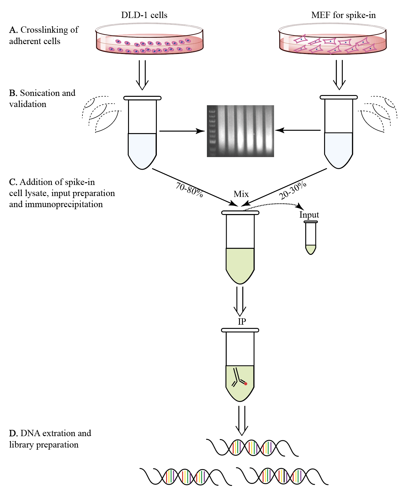
Figure 1. ChIP-Rx workflow. A. DLD-1 cells were crosslinked by formaldehyde solution and quenched by glycine B. After crosslinking, cells were sonicated in lysis buffer about 8 min, and the length of DNA fragments was validated by agarose gel electrophoresis (150-800 bp). C. Mix the sonicated spike-in cell lysate into sonicated experimental cell lysate. The input is prepared in advance, and the sonicated product is incubated with the antibodies to IP. D. Immunoprecipitated DNA was obtained and used for NGS library preparation.
 

A. Crosslinking of adherent cells

1. Prepare the cell (1 × 10⁷ cells ) in 15 cm dish with 20 mL medium.
2. Add 550 µL formaldehyde solution into above dish directly at the concentration of 1% and leave it on a shaker for 10 min at RT.
3. Add 1/20 volume of 2.5 M glycine into plates (final concentration is 0.125 M) to quench crosslinking and leave it on a shaker for 5 min at RT.
4. Rinse cells twice with cold PBS.
5. Harvest cells using scraper and transfer them into a 15 mL or 50 mL tube with PBS. 
6. Spin at 1500 g for 5 min at 4 °C and discard supernatant. 
7. Transfer pellets with 1 mL PBS into 1.5 mL EP tube. Spin at 1500 g for 3 min at 4°C and then remove the supernatant completely. 
8. Pellets can be flash-frozen at -80°C.
    

B. Sonication and validation

1. Suspend the cells with 1000 µL of ChIP Lysis buffer with protease and/or phosphatase inhibitors and transfer into two EP tubes（500 µL per tube）.
2. Sonicate for ~8 min for each sample (20 sec on, 59 sec off, 75% intensity，4°C).
3. Use 30 µL cell lysate to test the size of DNA fragments following steps 12-15.
4. Spin at 20,000 g for 15 min at 4°C to pellet debris.
5. Collect 20 µL supernatant and add 2 µL of 20 mg/mL Protease K. Mix and incubate at 65°C water bath for 120 min. 
6. PCR cleanup of step 5 sample.
7. Run sample for 18 min on 1.2% agarose gel to check sonication efficiency (150 V). The majority of DNA should be between 150 bp-800 bp. Sonicate further if necessary.
8. As soon as the validation was completed, spin down the sonicated sample at 20,000 g for 15 min at 4°C to pellet debris and collect the supernatant as chromatin sample.

C. Addition of spike-in cell lysate, input preparation and immunoprecipitation 

1. Measure the DNA concentration of the supernatant by nanodrop. Use ChIP Lysis buffer with protease and phosphatase inhibitors to adjust each chromatin sample into the same concentration.
2. Add 25% of spike-in chromatin into each sample and mix fully (Note: Operation conditions should be the same for DLD-1 cells and reference MEF cells. The two kind of cells were belong to the different species and own the similar epitopes).
3. Save 20 µL cell lysate as input DNA and store at -20°C. And the left supernatant was prepared for following IP.
4. Add 2-5 µg antibody into each IP sample and incubate at 4°C on rocker for overnight.
5. At the same time, 20-30 µL Magnetic Protein A/G beads for each sample was blocked with 1% BSA in PBS (freshly made or stored in -80°C) on rocker for overnight at 4°C. Then, wash beads with ChIP Lysis buffer twice. 
6. Resuspend beads in 50 µL ChIP Lysis buffer and transfer beads into the sample of step 20 for 2-4 h at 4°C on rocker.
7. Wash beads 3 times using 1mL High-salt Wash buffer per time. 
8. Wash beads twice using 1mL Low-salt Wash buffer per tim. 
9. Wash beads once with 1mL TEcontaining extra 50 mM NaCl per time. 
10. Add 200 µL ChIP Elution buffer containing extra 4 µL of 20 mg/ml Protease K into each IP sample. Mix and incubate at 65°C 3D thermal mixer for overnight.
11. At the same time, add 180 µL of ChIP Elution Buffer containing extra 4 µL of 20 mg/mL Protease K into above 20 µL input sample. Mix and incubate at 65°C 3D thermal mixer for overnight.

D. DNA extraction and library preparation

1. Add 200 µL 1 × TE buffer into each IP sample and each input sample. Then, add 400 µL of phenol: chloroform: isoamyl alcohol (P:C:IA) (lower layer) into each sample and shake vigorously for ~15 sec immediately.
2. Spin at maximal speed for 15 min at 4°C.
3. Transfer the upper aqueous layer to a new centrifuge tube containing 16 µL of 5 M NaCl , 1 µL of 5 µg/µL glycogen and 800 µL of ethanol. Then, mix well and incubate at -80°C for 30 min or overnight.
4. Spin at maximal speed for 15 min at 4°C to pellet DNA. Wash pellets by adding 800 µL of 70 % ethanol and spinning at maximal speed for 5 min at 4°C.
5. Discard the supernatant using 1-mL and 200-µL pipettes (NOT vacuum) carefully without disturbing the pellets. Spin the tubes briefly and remove any remaining liquid using 10-µL tips. Let the tubes air dry until pellets are just dry (~10 min). Do not over-dry. Pellets should still retain a moist appearance.
6. Resuspend each pellet in 20-50 µL of water. And quantify the DNA of each sample with Qubit 4 Fluorometer. Then, NGS library was established from 1-10 ng of above DNA using VAHTS^TM universal DNA library prep kit (10-13 cycles when PCR amplify step). 
7. Perform paired-end Illumina sequencing following the manufacturer’s instructions. 

DATA analysis (an example)

1. Check the quality of the raw read data in fastq format with Fastqc. The path of output results can be specified with the -o parameter.

            fastqc sample_R1.fq.gz -o sample_output

            fastqc sample_R2.fq.gz -o sample_output

2. Remove adaptors and low-quality reads. Trim Galore auto-detects whether the Illumina universal, Nextera transposase or Illumina small RNA adapter sequence was used. Here is an example for pair-end sequencing data.

            trim_galore -q 25 --phred33 --length 36 -e 0.1 --stringency 4 --paired -o trimmedFastq_dir sample_R1.fq.gz sample_R2.fq.gz > sample_trimmed.log 2>&1 &

3. Then the clean reads can be aligned to the experiment genome and reference exogenous genome (spike-in genome). In this protocal, Bowtie2 was used to align short reads to hg19 and mm10 assembly. The indexed genome can be downloaded online (http://bowtie-bio.sourceforge.net/bowtie2/index.shtml). The alignment results were further filtered based on their alignment quality by MAPQ filtering using samtools. The following command will align the pair-end input reads to the reference genome.

            (bowtie2 -p number_of_compute_cores_to_use -x reference_bowtie2_index -N 1 -1 sample_R1_val_1.fq.gz -2 sample_R2_val_1.fq.gz 2> sample_align.log) | samtools view -bS -F 3844 -f 2 -q 30 | samtools sort -O bam -@ number_of_compute_cores_to_use -o sample_reference.bam 

              samtools index sample_reference.bam

4. Remove PCR duplicates. Duplicates were marked and removed with Picard tools.

               picard MarkDuplicates -REMOVE_DUPLICATES True -I sample_reference.bam -O sample_reference.rmdup.bam -M sample_reference.rmdup.metrics

               samtools index sample_reference.rmdup.bam

5. Spike-in calibration. The normalization factor is calculated based on the assumption that the aligned read counts of the reference exogenous genome for each sample using the same number of cells are the same. So, we defined the scale factor α as:

Where N_spikein is the spike-in read counts of each sample, β is the scale factor used for normalizing the differences between IPs. Assuming the same mixing ratio among the experiments, we can derive β as: 

Where R is the mixing ratio or the mapping ratio between the experiment genome and reference exogenous genome of IP-corresponding input samples and R_{ref_input} is the mixing ratio for the selected reference sample. So, R can be calculated for each input samples as:

The aligned read counts for each sample was generated by samtools flagstat command. Here is an example:

            samtools flagstat sample_reference.rmdup.bam > sample_reference.rmdup.stat

            N =$(cat sample_ref.rmdup.stat | grep "total (QC-passed reads" | cut -d " " -f 1)

The detail can be referred from our online pipeline: https://github.com/FeiXavierChen-Lab/SPT5_2021/blob/main/01.1_ChIPseq_preprocessing.sh

6. Create coverage tracks and visualize results. Normalize the mapped reads to the scale factor using deeptools function bamCoverage with 1 bp bin size and remove the ENCODE Blacklist regions which can be downloaded from https://github.com/Boyle-Lab/Blacklist (Amemiya et al., 2019).

              bamCoverage -b sample_reference.rmdup.bam --binSize 1 --blackListFileName blacklist_file --normalizeUsing None –scaleFactor scalefactor --numberOfProcessors 23 -o sample.bw 2> sample.log

Tools like USCS and IGV allow displaying the overall mapping of reads and protein binding regions (Figure 2).
 

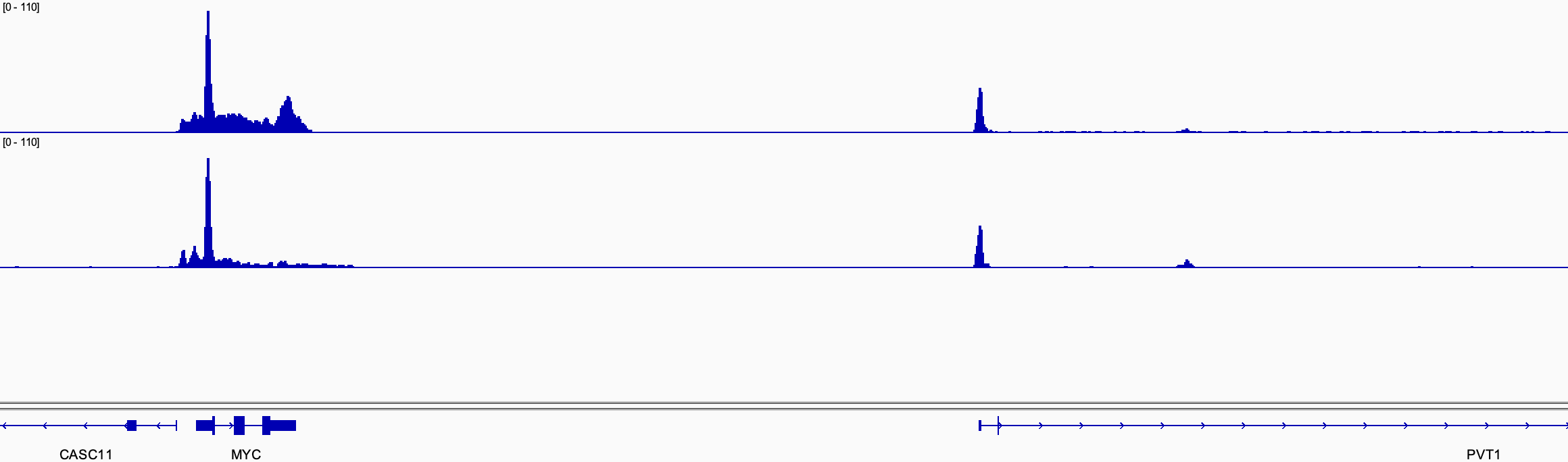
Figure 2. Track examples showing the occupancy of ChIP-Rx samples.
 

7. Plot heatmaps and meta-genes using DeepTools function plotHeatmap and plotProfile (Figure 3). Here is an example for generating the ChIP-Rx signal around TSS.

                  computeMatrix reference-point --referencePoint TSS -p 24 -b 3000 -a 3000 -R reference_TSS.bed -S bw_input bw_IP --binSize 100 --missingDataAsZero --skipZeros -o matrix_sample.gz

                  plotHeatmap -m matrix_sample.gz -out sample_Heatmap.pdf --colorList 'white,#173a55' –outFileSortedRegions sample.Heatmap.bed --missingDataColor "white" --refPointLabel TSS --samplesLabel input sample --sortUsingSamples 1 --heatmapHeight 28 --plotFileFormat pdf --dpi 720

                  plotProfile -m matrix_sample.gz --perGroup --refPointLabel TSS --samplesLabel input sample -out sample_Profile.pdf --plotHeight 16 --plotWidth 20
 

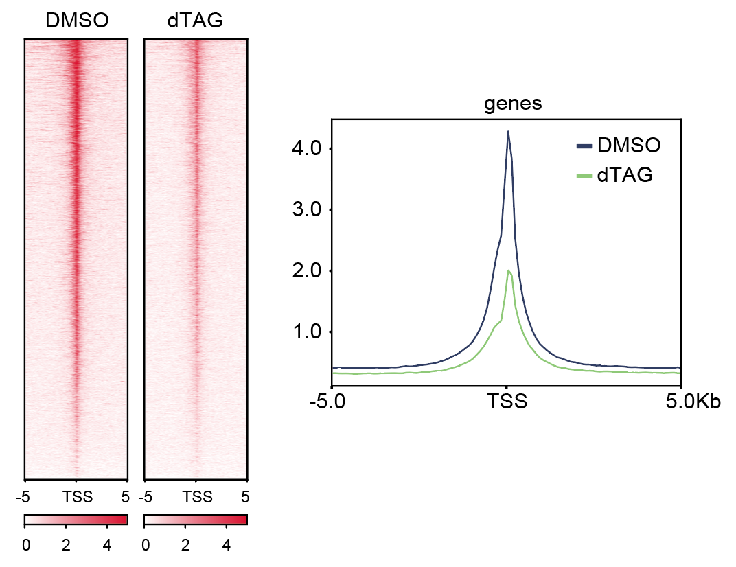
Figure 3. Examples of heatmaps and meta-genes showing the ChIP-Rx signal around TSS.

Recipes

1.  2.5 M Glycine

     Composition     total 50 mL

     Glycine              9.38 g

     H₂O                   to 50 mL

2. 1 M Tris-HCl (pH 8.0)

    Composition     total 1000 mL

    Tris-base           121.14 g

    HCl                    adjust pH to 8.0

    H₂O                   to 1000mL

3. 5 M NaCl

    Composition     total 1000mL

    NaCl                  292.2 g

    H₂O                   to 1000 mL

4. 0.5 M EDTA  pH 8.0

    Composition     total 1000 mL

    EDTA                 186.12 g

    NaOH                adjust pH to 8.0

    H₂O                   to 1000 mL

5. 10% DOC (Keep out light)

    Composition     total 50 mL

    DOC                   5 g

    H₂O                    to 50 mL

6. 10% SDS

   Composition     total 1000mL

   SDS                   100g

   H₂O                   to 1000 mL

7. 1 M HEPES (pH 7.4)

    Composition     total 1000 mL

    HEPES               238.3 g

    NaOH                adjust pH to 7.4

    H₂O                   to 1000 mL

8. Protease inhibitors (50 ×, stored at -20°C)

    Composition                        total 1 mL

    cOmplete Cocktail Tablets   1 tablet

    H₂O                                      to 1 mL

9. Phosphotase inhibitors (25 ×, stored at -20°C)

    Composition              total 1 mL

    PhosSTOP                  1 tablet

    H₂O                            to 1mL

10. ChIP Lysis buffer (stored at 4°C)

      Composition 

      50 mM HEPES (pH 7.4)

      150 mM NaCl

      2 mM EDTA (pH 8.0)

      0.1% DOC

      0.1% SDS

      Protease inhibitors 1 × (add before use)

      Phosphotase inhibitors 1 × (add before use)

11. High-salt Wash buffer (stored at 4°C)

      Composition

      20 mM HEPES (pH 7.4)

      500 mM NaCl

      1 mM EDTA (pH8.0)

      1.0% NP-40

      0.25% DOC

12. Low-salt Wash buffer

      Composition

      20 mM HEPES (pH 7.4)

      150 mM NaCl

       1 mM EDTA (pH 8.0)

       0.5% NP-40

       0.1% DOC

13. 1 × TE buffer 

      Composition

      10 mM Tris-HCl (pH 8.0)

       1 mM EDTA (pH 8.0)

14. ChIP Elution Buffer

     Composition

     50 mM Tris-HCl (pH 8.0)

     10 mM EDTA (pH 8.0)

     1.0% SDS

Acknowledgments

This work was supported by grants from the National Key R&D Program of China (2021YFA1301700), the National Natural Science Foundation of China (32070636), and the Shanghai Natural Science Foundation (20ZR1412100 and 22ZR1412400)

Competing interests

The authors declare that no competing interests exist.

References

D. A. Orlando, M. W. Chen, V. E. Brown, S. Solanki, Y. J. Choi, E. R. Olson, C. C. Fritz, J. E. Bradner, M. G. Guenther, Quantitative ChIP-Seq normalization reveals global modulation of the epigenome. Cell Rep. 9, 1163–1170 (2014)

Langmead, B., and Salzberg, S.L. (2012). Fast gapped-read alignment with Bowtie 2. Nat Methods 9, 357-359. 10.1038/nmeth.1923.

Li, H., Handsaker, B., Wysoker, A., Fennell, T., Ruan, J., Homer, N., Marth, G., Abecasis, G., Durbin, R., and Genome Project Data Processing, S. (2009). The Sequence Alignment/Map format and SAMtools. Bioinformatics 25, 2078-2079. 10.1093/bioinformatics/btp352.

Quinlan, A.R., and Hall, I.M. (2010). BEDTools: a flexible suite of utilities for comparing genomic features. Bioinformatics 26, 841-842. 10.1093/bioinformatics/btq033.

Ramirez, F., Ryan, D.P., Gruning, B., Bhardwaj, V., Kilpert, F., Richter, A.S., Heyne, S., Dundar, F., and Manke, T. (2016). deepTools2: a next generation web server for deep-sequencing data analysis. Nucleic Acids Res 44, W160-165. 10.1093/nar/gkw257.

Zhang, Y., Liu, T., Meyer, C.A., Eeckhoute, J., Johnson, D.S., Bernstein, B.E., Nusbaum, C., Myers, R.M., Brown, M., Li, W., and Liu, X.S. (2008). Model-based analysis of ChIP-Seq (MACS). Genome Biol 9, R137. 10.1186/gb-2008-9-9-r137.

Amemiya, H.M., Kundaje, A., and Boyle, A.P. (2019). The ENCODE Blacklist: Identification of Problematic Regions of the Genome. Sci Rep 9, 9354. 10.1038/s41598-019-45839-z.