Contribution of inter-relatedness chimpanzees to differential expression analysis

Detailed protocol: Contribution of inter-relatedness chimpanzees to differential expression analysis
 

Overview

A reader requested a detailed protocol for the Methods of our paper section titled “Contribution of inter-relatedness chimpanzees to differential expression analysis”. This section details how I analyzed our differential expression (DE) results to conclude that the contribution of inter-relatedness among some of our chimpanzees in our samples are fairly negligible towards our inter-species DE results. The original motivation for looking at the potential contribution of inter-relatedness to bias DE results came from a reviewer’s concern:

Anonymous reviewer said:
 

"I would like to see more discussion about the inter-relatedness of the
chimpanzees in the analysis of gene expression. Is that contributing to the
power of the DE analysis, which has really high numbers of DE genes..."
 

In primate research where samples are limited, the samples available to researchers may sometimes be related to one another. When doing interspecies DE analysis, this could in theory inflate the number of DE genes since the samples are not genetically independent and not representative to the species population as a whole. One could in theory account for this with more complicated models during the DE testing process (ie, a mixed model to account for genetic relatedness). However, our DE analysis methods did not account for that. So to address that concern, rather than change the DE analysis model, I used sub-sampling to emprically determine how utilizing inter-related chimps in our DE analysis pipeline (see detailed protocol for DE analysis) influences the number of DE genes discovered, compared to not using any inter-related chimps.

The results of this section are summarized in Fig1S3:
 

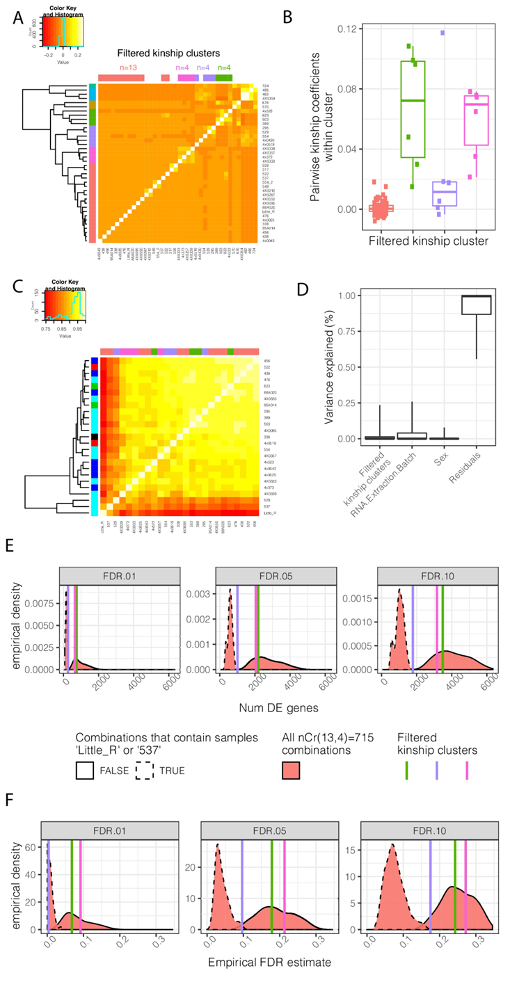
Figure Legend: Contribution of genetic relatedness to differential expression analysis between chimpanzee and human. (A) A mean-centered genetic relatedness/kinship matrix of the chimpanzee individuals used in DE analysis. Samples are hierarchically clustered and further grouped into k = 7 kinship clusters (row colors). The colors used to represent each cluster is consistent throughout the figure. These clusters were further manually filtered into three clusters of size n = 4 individuals with relatively high inter-relatedness and one cluster of size n = 13 individuals with relatively low inter relatedness (column colors). (B) The distribution of pairwise intra-cluster relatedness coefficients. The contribution of these cluster annotations as factors which explain gene expression and DE power is explored in C-F. (C) A clustered gene expression (log(RPKM)) Pearson correlation matrix. Row colors represent RNA extraction batch for RNA-seq. Column colors represent kinship cluster. (D) Variance partitioning analysis using a linear mixed model with each term as a mixed effect was used to quantify the contribution of various explanatory factors to expression of each gene. Boxplots indicate the fraction of variance explained by each factor for 0.05, 0.25, 0.5 0.75, and 0.95 percentiles across all expressed genes. As there is only one replicate per individual, a model term for individual was not appropriate, and individual effects are captured in the residual. (E) DE analysis was performed using n = 4 individuals each of chimpanzee and human. The effect of inter-related chimpanzee samples was assessed by all four chimpanzee individuals from one of the three highly inter-related clusters, or by drawing a combination of four individuals (without replacement) from the lowly inter-related cluster. The distribution of number of DE genes (E) across the resampled DE analyses is shown, as well as an empirical estimate of FDR based on the full n = 39 dataset (F). DE analyses containing outlier samples Little_R or 537, originating from the same technical batch, have a much larger effect on results than drawing from inter-related samples. Kinship matrix plotted in (A) is available as Figure 1—figure supplement 3—source data 1.
 

Data and code availability

In the remainder of this document, I will provide a bit detial of the analysis steps for this section. First, some notes on raw data and code availability:

• Publicly available raw data for this publication is described here,
• all code associated with this paper is in this git repository (but I make no promises on the cleanliness of my code!). This contains code that I used to go from raw data to partially processed and final figures displayed in the publication.
• Additionally, nitty details and R code for some of data exploration can be found on the website associated with that repo. Specifically, code for generating this Fig1S3 is fully detailed at this webpage and in the associated Rmarkdown used to create the webpage. Since all the partially processed data required to run that R code is included in the git repo, if you want to reproduce reproduce the image from R code, you just need to clone the repository (git clone https://github.com/bfairkun/Comparative_eQTL.git), then run that Rmarkdown document (analysis/20200907_Response_Point_06.Rmd)) with the analysis directory as the working directory. You may need to install packages and/or use the same R version I used to perfectly reproduce the code, and my R version and libraries can be found in detail at the bottom of the webpage.

Since all the R code is available in the Rmarkdown mentioned above, I will refrain from detailing R code here. Rather, I will explain the analysis steps behind FigS13, panel by panel, and mention relevant non-R code as needed…
 

Detailed Methods

Figure1S3A

Since the motivating question was to assess the contribution of inter-related chimpanzees, we first need to establish how the chimpanzee individuals in our cohort are related. To do so, we created a genetic relatedness matrix from the whole-genome-sequencing genotype data using GEMMA. GEMMA can take as input plink-bed files, and output a genetic relatedness matrix. More specifically, I did the following (Curly brackets denote placeholder filenames):

#Convert genotype data in vcf format to plink-bed format, while filtering for
#Minor allele frequency, genotyping rate, and hardy-weinberg equilibrium the
#--allow-extra-chr parameter is necessary to allow plink to recognize the
#chimpanzee chromosomes named 2A and 2B. This will create plink-bed  file named
#{output.prefix_name}.bed
plink --vcf {input.vcf} --vcf-half-call m --allow-extra-chr --geno 0 -recode12 \
--make-bed --out {output.prefix_name} --maf 0.05 --geno --hwe 1e-7.5

#use plink to identify snps in high-LD. Removing these snps from analysis is
#typically done before estimating genetic relatedness
plink --bfile PopulationSubstructure/plink/Merged --allow-extra-chr \
--indep-pairwise 50 5 0.5

#Use plink extract the independent snps from the original plink-bed file into a
#new bedfile named {output.prefix_name_pruned}.bed
plink --bfile {output.prefix_name} --allow-extra-chr --extract \
plink.prune.in --make-bed --out {output.prefix_name_pruned}

#Use gemma to create a relatedness matrix
#This should output a file named GRM.cXX.txt, which is the genetic relatedness
#matrix pictured in Fig1S3A
gemma -gk 1 -bfile {out.prefix_name_pruned} -o GRM

This genetic related matrix (GRM) details how related each individual is to every other individual. Often, GRM use a coefficient of 0.5 to indicate genetic relatdenss equivalent to a 1st degree relationships (ie parent:child or sibling relationships), 0.25 for 2nd degree relationships, etc (see Fig6S2). Or for whatever reason, the scale of the GEMMA coefficients seem to be halved. Also, in our case, for mathemical reasons, we asked gemma to output a mean-centered matrix (available here or as fig1-figsupp3-data1-v2), meaning that the coefficients are centered around 0. In any case, what is really relevant for this is that bigger numbers correspond to more relatedess between two individuals. In Fig1S3A, you can see occasional pairs of related individuals, which in Fig6S2 we show matches with what we expect from pedigree information. We also see a few clusters of groups of related individuals. I thought these could be particularly useful towards answering our original question: “Does inter-relatedness contribute meaningfully to our inter-species DE comparisons”. More specifically, I thought that I could perform DE analysis with 4 humans and 4 chimps (where the 4 chimps do not show any inter-relatedness) and compare it to another DE analysis where the 4 chimps are selected from one of those clusters of highly inter-related chimps. Sample size of 4 chimps and 4 humans was chosen only because it seems there aren’t many obvious clusters of related chimps larger than 4 individuals.

Even though you can visually see these few clusters of highly inter-related chimps, I decided to use R to do some clustering to pick out the clusters I naturally saw by eye in the heatmap matrix in Fig6S2A. I therefore did clustering with k=7 clusters, resulting in the 7 clusters colored on the rows of the heatmap. Manual visual inspection of these clusters, I noticed that the clusters in pink, purple, and green had about 4 inter-related individuals each. Meanwhile, the orange cluster contained mostly unrelated individuals. I figured these could serve as my comparisons:

• The pink, purple, and green clusters are all different ‘replicates’ of highly inter-related chimpanzees that I could perform a DE analysis with, and compare it to
• A DE analysis with orange cluster which has mostly unrelated individuals.

But first, I felt I needed to ‘clean up’ the orange cluster of unrelated individuals a bit… Even though most samples are unrelated, there are still clearly a couple of pairs that are related. And also, the purple cluster has 5 individuals while the pink and green cluster had 4. I was envisioning performing DE analysis using 4 within-cluster-chimp indivuals and 4 human individuals to be consistent. So I manually redefined these clusters by the following criteria:

• pink cluster was left as is, with 4 highly inter-related individuals
• green cluster was left as is, with 4 highly inter-related individuals
• purple cluster was pruned from 5 to 4 indivudals, by dropping the sample 4x0430 which had lowest average relatedness to the other individuals in that cluster
• the orange cluster was pruned from 19 to 13 individuals, by dropping all individuals which had a pairwise relatedness coefficient to any other individual in that cluster that is over 0.05.

These refined cluster defintions are shown as the column colors over the heatmap

Figure1S3B

This plot shows the all the pairwise relatedness coefficeints among samples within each of the refined clusters I described above. In summary, I grouped the chimpanzee individuals to be used in DE analysis into 4 clusters: - a pink cluster with 4 highly inter-related individuals - a green cluster with 4 highly inter-related individuals - a purple cluster with 4 highly inter-related individuals - a orange cluster with 13 un-related individuals

I will perform a DE analysis using the pink cluster individuals as the 4 chimpanzee individuals, and compare the results to a DE analysis where I sample 4 individuals from the orange cluster as the chimpanzee individuals in the inter-species comparison. I will do the same for the green and purple cluster.

Figure1S3C

Before performing a DE analysis, it is important to do some checks. Here, I created a gene-expression Pearson correlation matrix for all the samples in the refined clusters which I will eventually use in DE analysis. What sticks out is the presence of two relative outlier samples in the lower left (samples 537 and Little_R, both in the orange cluster, as shown on the heatmap column colors). Though these two individuals are not related, they seem to cluster together. And generally, it doesn’t seem that the inter-related individuals cluster together in this gene-expression correlation matrix. I therefore wondered of other, technical factors may explain the observed gene-expression clustering patterns. For example, I hypothesize that the RNA extraction batch (these samples were collected in 5 or 6 batches in total) may introduce some technical effects that cause samples within the same batch to cluster closer together. I colored the RNA-extraction batch for each sample on the rows of the heatmap. Although the RNA-extraction batch doesn’t clearly explain all of the clustering patterns, it might be useful to use a more principled procedure to evaluate the relative contribution of relatedness versus RNA-extraction batch or other features to explain similarity among samples.

Figure1S3D

To evaluate the relative contribution of relatedness and batch to gene expression patterns among the chimp individuals, I used the VariancePartition R package to implement a linear mixed model to explain gene expression patterns among these chimp individuals. Specifically, the variancePartition package was used to implement a linear model for each gene, with random effects terms for sex, RNA extraction batch, and which refined relatedness cluster each individual belongs to (orange, purple, green or pink). I more or less implemented this by following the standard application vignette section 2.1 in the VariancePartition manual. Again, my code for this section is available in the abovementioned Rmarkdown. The variance explained by each term is plotted, as boxplot for the distribution for each model across all genes. The main conclusion is that the RNA extraction batch explains more variation than the relatedness cluster. Note that since there are no replicates for any individual, it would not be appropriate to include a term for individual in the model, and any individual effects are captured in the residual.

Figure1S3E.

Finally, to empirically assess the contribution of inter-relatedness to our interpsecies DE results, I performed DE analysis using the protocol described in detail here. I performed 4 DE contrasts, each with 4 chimpanzee individuals as detailed below, and 4 human individuals randomly selected amongst the human samples originally described in Pavlovic et al. The 4 human samples were selected randomly, but always kept the same amongs the following 4 DE contrasts:

1. Pink cluster chimps vs human
2. Purple cluster chimps vs human
3. Green cluster chimps vs human
4. Orange cluster chimps vs human

If the use of inter-relatedness impacts DE results substantially, I expect contrasts 1-3 to have many more DE genes that contrast 4, though many of them I expect to be false positives that are just driven by the gene expression levels that are specific to the inter-related cluster os chimps but not to chimpanzee species as a whole. Note that since the orange cluster has 13 samples, we could choose any 4 of them for this contrast. In effect, a single sampling of 4 our of 13 individuals in this cluster is just one realization of the sampling distribution. So I mine as well perform contrast 4 with every possible combination of the 13 samples. That is, there are 715 ways to choose 4 individuals from the 13 individuals in the orange cluster (“4 choose 13”), and I mine as well perform contrast 4 in all of those possible ways to get a distribution of results for that contrast. This creates sort of a “null” distribution out of contrast 4, from which we can compare contrasts 1-3.

After performing the DE analysis for those 4 contrasts, I plotted the results. At various FDR thresholds, I plotted the number of DE genes identified in each contrast. Interestingly, I noted that the “null” distribution of contrast4 looked bimodal, where some iterations of contrast4 had very many significant DE genes, while other iterations had very few. I eventually realized that this is due to the presence of at least one of those outlier samples mentioned above (Little_R or 537) included in the DE analysis. That is, when one of those outlier samples happens to be chosen, you get way less DE genes. Arguably, these two outlier samples should be dropped from the orange cluster entirely, since they are outliers amongst all samples. Rather than drop those samples completely, I presented the combinations of results for contrast4 broken into two distributions: the iterations that included one of those outlier samples versus the iterations that did not include those samples.

What I see is that the contrast1 & contrast3 mostly overlap the distribution of contrast4 (at least when you do not include the outlier samples). And contrast2 if anything has less DE genes than contrast4 distribution.

In summary, when I took groups of inter-related chimps and performed DE analysis, you get about the same number of DE genes as if you take a group of unrelated chimps and perfom DE analysis.

Figure1S3F

This is the same as Figure1S3E except that now I am plotting an estimate of FDR rate. That is, similar to Fig1S2B, I performed DE analysis with all 39 chimp and 39 human samples to obtain the FDR<0.01 ‘gold standard’ set of DE genes which I assert to represent ground truth. Then, in the 4 contrasts mentioned above, I look at what genes were identified as DE (at FDR<0.01, FDR<0.05, or FDR<0.1) and assess what fraction of significant genes were truly DE according to ground-truth. I am calling that the empirical false discovery rate. Again, I find that the contrasts1-3 of inter-related chimps do not seem to have a higher empirical FDR rate than the distribution of results from combinations of contrast4.

Category