
- Home
- Protocols

-

Transformation, Normalization, and Batch Effect Removal
Published: Jul 20, 2022 DOI: 10.21769/BioProtoc.4462 Views: 6711
Edited by: Ruidong Li Reviewed by: Yinqi ZhaoMeiyue Wang
Abstract
In bulk RNA-seq analysis, normalization and batch effect removal are two procedures necessary to scale the read counts and reduce technical errors. Many differential expression analysis tools require a raw count matrix as input and embed the normalization and batch effect removal procedures in the analysis pipeline. However, researchers need to perform these two procedures independently when they build up their own bulk RNA profile analysis models. This protocol includes detailed codes and explanations for normalization and batch effect removal, helping users to more conveniently understand and perform these procedures. In this case study, we use the easily obtainable Arabidopsis thaliana bulk RNA-seq dataset, so that researchers interested in this topic can use this protocol to learn and apply.
Keywords: TranscriptomeBackground
RNA-seq is a widely used sequencing technique that reveals the quantity of gene expression. Based on RNA-seq reads, we can perform quality control and alignment, getting a raw count matrix that notes expression counts for each gene, in each sample. In practice, technical errors in the raw count matrix may affect the downstream analysis. Therefore, we should apply normalization and batch effect removal procedures to correct this technical bias.
RNA-seq measures gene expression based on the number of reads aligned to the gene. The number of reads aligned to the reference is considered as a random variable, but experimental errors, such as ununified fragment amplification and different coverage, can affect the read count. Additionally, gene length can affect the alignment—long genes have a higher probability to get reads align, while short genes have the opposite issue. Therefore, a normalization procedure is necessary in RNA-seq analysis, to make the read counts comparable across samples. The standard normalization methods include library size normalization and gene length normalization. The former focuses on making the library sizes comparable by scaling raw read counts in each sample by a single sample-specific factor, reflecting its library size. Gene length normalization corrects the impact of gene length on the estimation of gene abundances. Accounting for gene length is necessary when comparing expression between different genes within the same sample.
While normalization focuses on correcting the bias generated in each sequencing experiment, batch effect removal helps to reduce the bias generated across batches. Batches may include the dates of sequencing, people who performed the sequencing, the protocol, the type of sequencing machine, etc. When sequencing is performed in different batches, the systematic technical differences can cause a non-biological bias that should be considered in RNA-seq analysis. When removing batch effects, two situations may occur: (i) the batch information is known, or (ii) the batch information is unknown. Different batch effect removal procedures should be used under each situation.
Both normalization and batch effect removal procedures aim to reduce technical bias, but they work on different aspects. This protocol shows readers how to perform different normalization and batch effect removal methods in the case study section, using two R packages: edgeR (Robinson et al., 2010; McCarthy et al., 2012) and sva (Leek et al., 2014) with limma (Ritchie et al., 2015), respectively.
Software
All the software can be downloaded/used from the following locations:
R (Version 4.1) https://www.r-project.org/
Package edgeR (Version 3.34.0) https://bioconductor.org/packages/release/bioc/html/edgeR.html
Package sva (Version 3.40.0) https://bioconductor.org/packages/release/bioc/html/sva.html
Package limma (Version 3.48.0) https://bioconductor.org/packages/release/bioc/html/limma.html
Input data
To demonstrate different normalization and batch effect removal methods, we use the Arabidopsis thaliana RNA count data published by Cumbie et al. ( 2011) as an example. Summarized count data is available as an R dataset, and readers can download the data using the link http://bioinf.wehi.edu.au/edgeR/UserGuideData/arab.rds. In Cumbie’s experiment, they inoculated six-week-old Arabidopsis plants with the ΔhrcC mutant of P. syringae. Control plants were inoculated with a mock pathogen. Each treatment was done as biological triplicates, with each pair of replicates at separate times and derived from independently grown plants and bacteria.
We can use the following script to download and import the input dataset in R (or R studio) environment:
# Specify URL where the file is stored
url <- "http://bioinf.wehi.edu.au/edgeR/UserGuideData/arab.rds"
# Specify destination where file should be saved
destfile <- "path/to/folder/arab.rds"
# Apply download.file function in R
download.file(url,destfile)
# Import the input r dataset
raw_counts_matrix <- readRDS(destfile)
# Check out the import raw counts matrix
head(raw_counts_matrix)
| mock1 | mock2 | mock3 | hrcc1 | hrcc2 | hrcc3 | |
| AT1G01010 | 35 | 77 | 40 | 46 | 64 | 60 |
| AT1G01020 | 43 | 45 | 32 | 43 | 39 | 49 |
| AT1G01030 | 16 | 24 | 26 | 27 | 35 | 20 |
| AT1G01040 | 72 | 43 | 64 | 66 | 25 | 90 |
| AT1G01050 | 49 | 78 | 90 | 67 | 45 | 60 |
| AT1G01060 | 0 | 15 | 2 | 0 | 21 | 8 |
Case study
Normalization
# Load library
library(edgeR)
# Create group vector that indicate each sample’s group type
group <- c('mock','mock','mock','hrcc','hrcc','hrcc')
# Create DEGList object
DEGL <- DGEList(counts=raw_counts_matrix, group=group)
# Checkt out DEGList object
DEGL> DEGL
An object of class "DGEList"
$counts
26217 more rows ...mock1 mock2 mock3 hrcc1 hrcc2 hrcc3 AT1G01010 35 77 40 46 64 60 AT1G01020 43 45 32 43 39 49 AT1G01030 16 24 26 27 35 20 AT1G01040 72 43 64 66 25 90 AT1G01050 49 78 90 67 45 60
$samplesgroup lib.size norm.factors mock1 mock 1902162 1 mock2 mock 1934131 1 mock3 mock 3259861 1 hrcc1 hrcc 2130030 1 hrcc2 hrcc 1295377 1 hrcc3 hrcc 3526743 1 Based on the input raw count matrix, we can perform different normalization methods. The most commonly used methods include library size normalization and gene length normalization (Abbas-Aghababazadeh and Li, 2018). Library size normalization divides each column of the raw count matrix by a normalization factor estimated by other samples. Recently proposed library size normalization methods are the trimmed mean of M-values (TMM), relative log estimate (RLE), and upper quartile (UQ). Gene length normalization methods include reads/fragments per kilobase of exon per million reads/fragments mapped (RPKM/FPKM), and transcripts per kilobase million (TPM). In the edgeR package, the first step is to create a DEGList object, which includes the count matrix and group information.
Counts per million (CPM)
The simplest way to normalize the data is to convert raw counts to counts per million (CPM). It divides every count in a sample by the total number of counts for that sample multiplied by 106.
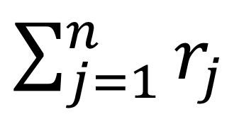
For each sample,
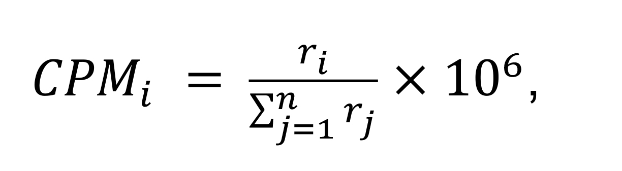
Where i is the ith feature (gene), ri represents the count number, and n is the total number of genes. Note that CPM normalization keeps the raw library size for each sample and does not scale library size. In the edgeR package, the function calcNormFactors() performs library normalization on the input DEGList object. If we set parameter method = "none", the function will not scale the library size, and will directly use each sample’s total read counts as library size. We can get the cpm matrix via function cpm(). Additionally, we can set log = TRUE in the cpm() function, to calculate the log2(CPM).
# Keep the raw library size
DEGL_cpm <- calcNormFactors(DEGL, method = "none")
# Calculate the cpm
cpm <- cpm(DEGL_cpm, log = FALSE, normalized.lib.sizes=TRUE)
# Calculate the log cpm
log_cpm <- cpm(DEGL_cpm, log = TRUE, normalized.lib.sizes=TRUE)
#Check out the cpm normalized matrix and log cpm normalized matrix
head(cpm)
head(log_cpm)> head(cpm)
> head(log_cpm)mock1 mock2 mock3 hrcc1 hrcc2 hrcc3 AT1G01010 18.400115 39.811161 12.2704618 21.59594 49.40647 17.012864 AT1G01020 22.605856 23.266263 9.8163695 20.18751 30.10707 13.893839 AT1G01030 8.411481 12.408673 7.9758002 12.67588 27.01916 5.670955 AT1G01040 37.851666 22.232207 19.6327389 30.98548 19.29940 25.519296 AT1G01050 25.760161 40.328189 27.6085391 31.45496 34.73892 17.012864 AT1G01060 0.000000 7.755421 0.6135231 0.00000 16.21150 2.268382 mock1 mock2 mock3 hrcc1 hrcc2 hrcc3 AT1G01010 4.267107 5.345726 3.7142054 4.488650 5.651355 4.159228 AT1G01020 4.552132 4.592183 3.4155622 4.395177 4.952390 3.882448 AT1G01030 3.211894 3.729319 3.1424103 3.758095 4.800812 2.706009 AT1G01040 5.274478 4.528969 4.3566298 4.992751 4.332963 4.721014 AT1G01050 4.734130 5.363953 4.8309999 5.013869 5.153524 4.159228 AT1G01060 -0.227364 3.105947 0.5535731 -0.227364 4.093025 1.642735 Trimmed mean of M-values (TMM) normalization
TMM is a weighted trimmed mean of M-values (to the reference) library size normalization method, which was proposed by Robinson and Oshlack (2010). This method assumes that most genes are not differentially expressed, accounting for library size variation between samples. We set parameter method = "TMM" in calcNormFactors() function, to calculate the library size normalization factor for each sample. Then, we can calculate the CPM based on TMM scaled library size.
# Calculate normalization factors using TMM method to align columns of a count matrix
DEGL_TMM <- calcNormFactors(DEGL, method="TMM")
# Calculate the cpm with the TMM normalized library
TMM <- cpm(DEGL_TMM, log = FALSE, normalized.lib.sizes=TRUE
# Check out the cpm of TMM normalization
head(TMM)
> head(TMM)mock1 mock2 mock3 hrcc1 hrcc2 hrcc3 AT1G01010 17.69333 37.512585 13.8788097 21.03330 43.29289 19.451664 AT1G01020 21.73752 21.922939 11.1030477 19.66157 26.38160 15.885526 AT1G01030 8.08838 11.692234 9.0212263 12.34563 23.67580 6.483888 AT1G01040 36.39771 20.948586 22.2060955 30.17822 16.91128 29.177496 AT1G01050 24.77066 37.999761 31.2273218 30.63546 30.44031 19.451664 AT1G01060 0.00000 7.307646 0.6939405 0.00000 14.20548 2.593555 Relative log expression (RLE) normalization
The RLE normalization method was proposed by Anders and Huber (2010). A median library is calculated from the geometric mean of all columns, and the median ratio of each sample to the median library is taken as the scale factor. This is the default normalization method in R package DESeq (Love et al., 2014), adapted for use with edgeR. In the calNormFactors() function, we can set method = "RLE" to calculate the scale factor, and then get the CPM based on the RLE normalized library size.
# Calculate normalization factors using RLE method to align columns of a count matrix
DEGL_RLE <- calcNormFactors(DEGL, method="RLE")
# Calculate the cpm with the RLE normalized library
RLE <- cpm(DEGL_RLE, log = FALSE, normalized.lib.sizes=TRUE)
# Check out the TMM normalized result
head(RLE)> head(RLE)mock1 mock2 mock3 hrcc1 hrcc2 hrcc3 AT1G01010 18.610636 38.777094 13.3567455 20.48292 45.59497 18.124818 AT1G01020 22.864495 22.661938 10.6853964 19.14708 27.78443 14.801935 AT1G01030 8.507719 12.086367 8.6818846 12.02259 24.93475 6.041606 AT1G01040 38.284736 21.654741 21.3707928 29.38854 17.81053 27.187227 AT1G01050 26.054890 39.280692 30.0526773 29.83383 32.05896 18.124818 AT1G01060 0.000000 7.553979 0.6678373 0.00000 14.96085 2.416642 Upper Quartile (UQ) normalization
The UQ normalization, proposed by Bullard et al. (2010), calculates the scale factors from the 75% quantile of the counts for each library. Like TMM and RLE normalization, we can set the method = “upperquartile” to perform UQ normalization, and then get the CPM counts.
# Calculate normalization factors using UQ method to align columns of a count matrix
DEGL_UQ <- calcNormFactors(DEGL, method="upperquartile")
# Calculate the cpm with the UQ normalized library
UQ <- cpm(DEGL_UQ, log = FALSE, normalized.lib.sizes=TRUE)
# Check out the UQ normalized result
head(UQ)
> head(UQ)mock1 mock2 mock3 hrcc1 hrcc2 hrcc3 AT1G01010 19.012345 39.266313 13.506840 20.16548 44.42250 18.063364 AT1G01020 23.358024 22.947845 10.805472 18.85034 27.06996 14.751748 AT1G01030 8.691358 12.238851 8.779446 11.83626 24.29355 6.021121 AT1G01040 39.111111 21.927941 21.610944 28.93307 17.35254 27.095046 AT1G01050 26.617284 39.776265 30.390390 29.37145 31.23457 18.063364 AT1G01060 0.000000 7.649282 0.675342 0.00000 14.57613 2.408449
Reads per kilobase of exon per million reads mapped, and fragments per kilobase of exon per million mapped fragments normalization (RPKM and FPKM)
RKPM is a within-sample normalization method, and it is used to compare gene expression levels within a single sample. FPKM is analogous to RKPM, but it is explicitly used in paired-end RNA-seq experiments (Trapnell et al., 2010).
For each sample,
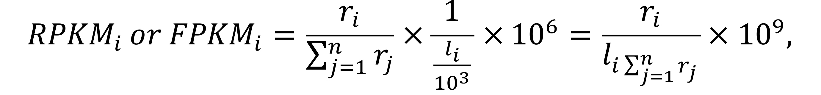
where i is the ith feature (gene) counts, ri represents the count’s number, n is the total number of features, and li is the length of the gene i.
RPKM/FPKM normalization needs the length for each feature, so we should download the dataset of each gene’s length first, and then add it into the DEGList object for the following steps. Here, we use the TxDb.Athaliana.BioMart.plantsmart28 database, to calculate each gene’s length, and then use the function rpkm() to perform RPKM normalization.
# Download the TxDb and import the database into R
BiocManager::install("TxDb.Athaliana.BioMart.plantsmart28")
# Import the database into R environment and create a database variable
library(TxDb.Athaliana.BioMart.plantsmart28)
TxDb <- TxDb.Athaliana.BioMart.plantsmart28
# Subtract the gene length information from TxDb.Athaliana.BioMart.plantsmart28
ref_gene_length <- as.data.frame(genes(TxDb))["width"]
# Delete the genes that in raw counts matrix without length information in reference
raw_counts_matrix <- raw_counts_matrix[intersect(rownames(raw_counts_matrix), rownames(ref_gene_length)),]gene_length <- ref_gene_length[rownames(raw_counts_matrix),]
# Create a DEGList with the gene length information
DEGL_with_gene_length <- DGEList(counts=raw_counts_matrix, group=group, genes=data.frame(Length=gene_length))
# Check out the DEGList with gene length information
DEGL_with_gene_length
# Calculate normalization factors to align columns of a count matrix
DEGL_with_gene_length_rpkm <- calcNormFactors(DEGL_with_gene_length)
# Calculate RPKM normalization
RPKM <- rpkm(DEGL_with_gene_length_rpkm)
# Check out the RPKM normalized matrix
head(RPKM)> head(RPKM)mock1 mock2 mock3 hrcc1 hrcc2 hrcc3 AT1G01010 7.801623 16.550845 6.1202305 9.281576 19.050395 8.5746344 AT1G01020 7.739512 7.810344 3.9535383 7.005845 9.373824 5.6544272 AT1G01030 3.916887 5.665586 4.3690329 5.983177 11.441850 3.1390522 AT1G01040 4.505729 2.594858 2.7491815 3.738725 2.089198 3.6109587 AT1G01050 12.491248 19.174183 15.7486426 15.460784 15.318963 9.8063737 AT1G01060 0.000000 1.628241 0.1545382 0.000000 3.156759 0.5773676 Transcripts per kilobase million (TPM) normalization
TPM, introduced by Li et al. (2010), is closely correlated with RPKM/FPKM normalization. To better demonstrate their correlation, we show their expressions as below:
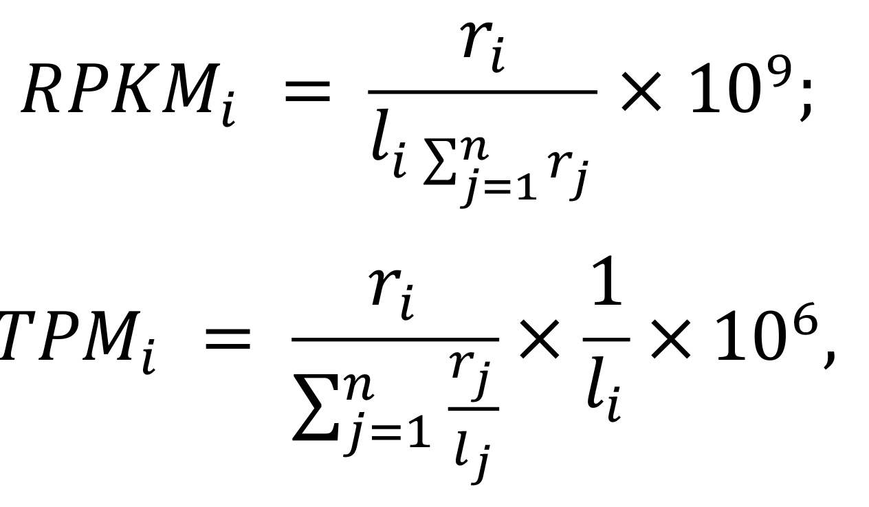
Where i is the ith feature, ri represents the count's number, li represents the length of the gene, and
 is the total number of read counts. We can convert the RPKM values to TPM by the following equation:
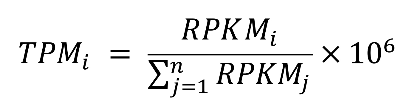
To perform the TPM normalization, we need to create a self-defined function rpkm_to_tpm().
# Calculate TPM from RPKM
# Input: RPKM normalized matrix
# Output: TPM normalizaed matrix
rpkm_to_tpm <- function(x) {
rpkm.sum <- colSums(x)
return(t(t(x) / (1e-06 * rpkm.sum)))
}Then, apply rpkm_to_tpm() to perform TPM normalization, based on RPKM normalization results.
# Use the constructed function perform tpm normalization based on the result of RPKM normalization
TPM <- rpkm_to_tpm(RPKM)
# Check out the TPM normalization result
head(TPM)
> head(TPM)mock1 mock2 mock3 hrcc1 hrcc2 hrcc3 AT1G01010 12.583074 27.187909 8.6959745 15.640215 35.142449 12.684487 AT1G01020 12.482896 12.829974 5.6174138 11.805422 17.291984 8.364614 AT1G01030 6.317465 9.306803 6.2077725 10.082142 21.106891 4.643611 AT1G01040 7.267196 4.262547 3.9061947 6.300057 3.853965 5.341704 AT1G01050 20.146872 31.497241 22.3765744 26.052687 28.259039 14.506603 AT1G01060 0.000000 2.674696 0.2195767 0.000000 5.823303 0.854102
Batch effect removal
RNA-seq experiments are often produced in multiple batches because of logistical or practical restrictions, which cause technical variation and differences across batches. We call the bias caused by the non-biological factor from different batches as batch effects (Leek et al., 2010). Proposed batch effect removal methods include ComBat (Johnson et al., 2007) with known sources effects, and SVA seq (Leek, 2014) or RUV seq (Risso et al., 2014) for heterogeneity from unknown sources. Meanwhile, commonly used R packages, such as edgeR and DESeq2, include batch variables in the linear model, to perform differential gene expression analysis.
Here, we use R package sva in the case study. This package, which includes the functions ComBat, ComBat-seq, and sva, can remove batch effects in two ways: (i) directly removing known batch effects, and (ii) identifying and estimating surrogate variables from unknown sources in RNA-seq experiments.
Remove batch effects with known batches based on ComBat function
ComBat removes the batch effect in datasets where the batch covariate is known. Users can choose parametric or non-parametric empirical Bayes frameworks for adjusting data for batch effects. Function ComBat() returns the adjusted RNA expression data based on a cleaned and normalized input counts matrix. Here, we use the TMM-CPM normalized expression profile (a result from section 1.2) as an input dataset for ComBat.
# Import the sva package
library(sva)
# Create batch vector
batch <- c(1,2,3,1,2,3)
# Apply parametric empirical Bayes frameworks adjustment to remove the batch effects
combat_edate_par = ComBat(dat=TMM, batch=batch, mod=NULL, par.prior=TRUE, prior.plots=TRUE)
# Apply non-parametric empirical Bayes frameworks adjustment to remove the batch effects
combat_edata_non_par = ComBat(dat= TMM, batch=batch, mod=NULL, par.prior=FALSE, mean.only=TRUE)
# Check out the adjusted expression profiles
head(combat_edate_par)
head(combat_edate_non_par)
> head(combat_edate_par)
> head(combat_edata_non_par)mock1 mock2 mock3 hrcc1 hrcc2 hrcc3 AT1G01010 23.32251 25.051220 22.3741482 26.00493 28.79416 26.943792 AT1G01020 20.57127 18.369262 16.9645376 18.85090 21.38939 20.798486 AT1G01030 10.02911 8.658437 12.7601412 13.54820 16.20375 10.275468 AT1G01040 29.55215 26.740817 23.0471627 24.93558 23.85726 28.751158 AT1G01050 26.66558 32.188893 33.2713853 31.45122 26.86053 24.073241 AT1G01060 0.00000 7.307646 0.6939405 0.00000 14.20548 2.593555 mock1 mock2 mock3 hrcc1 hrcc2 hrcc3 AT1G01010 22.477138 23.049996 21.5636368 25.81711 28.83030 27.136491 AT1G01020 21.106413 18.092070 16.0590482 19.03046 22.55073 20.841526 AT1G01030 9.348134 7.539353 11.9653553 13.60539 19.52292 9.428017 AT1G01040 30.843475 26.446379 22.5551441 24.62398 22.40908 29.526545 AT1G01050 25.910028 34.560019 33.9462917 31.77483 27.00057 22.170634 AT1G01060 0.000000 7.307646 0.6939405 0.00000 14.20548 2.593555 Remove batch effects with known batches based on ComBat_seq function
ComBat_seq (Zhang et al., 2020) is an improved model from ComBat that uses negative binomial regression, being explicitly designed for RNA-seq studies. Similarly to ComBat, ComBat_seq requires known batches information, but it uses a raw count matrix as input, instead of normalized data. ComBat_seq returns the adjusted integer counts matrix.
# Include group condition
combat_seq_with_group <- ComBat_seq(raw_counts_matrix, batch=batch, group=group, full_mod=TRUE)
# Without group condition
combat_seq_without_group <- ComBat_seq(raw_counts_matrix, batch=batch, group=NULL, full_mod=FALSE)
# Check out the adjusted expression profiles
head(combat_seq_with_group)
head(combat_seq_without_group)> head(combat_seq_with_group)
> head(combat_seq_without_group)mock1 mock2 mock3 hrcc1 hrcc2 hrcc3 AT1G01010 42 41 64 55 35 97 AT1G01020 38 33 51 38 28 79 AT1G01030 18 15 43 29 21 31 AT1G01040 54 52 70 49 31 103 AT1G01050 50 61 120 67 35 76 AT1G01060 0 15 2 0 21 8 mock1 mock2 mock3 hrcc1 hrcc2 hrcc3 AT1G01010 41 40 68 55 36 93 AT1G01020 39 32 54 38 29 75 AT1G01030 16 17 45 30 20 30 AT1G01040 55 52 75 48 30 100 AT1G01050 46 62 110 71 32 88 AT1G01060 0 15 2 0 21 8 Both ComBat and ComBat_seq functions can remove the batch effects when we know the batch information. When this is not the case, we can use the sva method to remove unknown batch effects in the count matrix.
Remove batch effects with unknown batches based on sva function
For the Arabidopsis thaliana RNA-seq study, we assume there is no batch information or adjustment information, so we need to use the sva method to correct the gene expression profile. First, the complete model matrix needs to be created, including the adjustment variables and the variable of interest (treatment). In this case, we do not have adjustment variables, and the variable of interest is binary (mock or hrcc). Therefore, we treat the variables of interest as factor variables, and create the full model matrix mod:
# Create the group variable in data frame format
df_group <- as.data.frame(group)
rownames(df_group) <- c("mock1","mock2","mock3","hrcc1","hrcc2","hrcc3")
colnames(df_group) <- "Treatment"
# Create the full model matrix mod
mod = model.matrix(~as.factor(Treatment), data=df_group)The null model matrix should only contain the adjustment variables. We assume there are no adjustment variables, so the null model matrix should be an all-ones vector.
# Create the null model matrix
mod0 = model.matrix(~1,data=df_group)# Create the null model matrixmod0 = model.matrix(~1,data=df_group)Now that the full model matrix and null model matrix are created, we can apply the sva function, to estimate the batch and get the sv object. The sva function can identify the number of latent factors that need to be estimated, and then return the sv object.
# Calculate the sv object
sva_result <- sva(TMM,mod,mod0)
names(sva_result)
> names(sva_result)
[1] "sv" "pprob.gam" "pprob.b" "n.sv"The sva function returns a list composed by four variables—sv, pprob.gam, pprob.b, and n.sv—where sv is a matrix whose columns correspond to the estimate surrogate variables, pprob.gam is the posterior probability that each gene is associated with one or more latent variables, pprob.b is the posterior probability that each gene is associated with the variable of interest, and n.sv is the number of surrogate variables estimated by the sva. Each of the return variables has a specific usage in the downstream analysis. In this case study, we are only focusing on removing the batch effects, and we can use the removeBatchEffect() function from limma to achieve this goal.
Result interpretation
In Figure 1 we created the log2(CPM) violin plot of raw counts and used five normalization methods (RLE, RPKM, TMM, TPM, and UQ). The values of log2(CPM) obtained from library size normalization methods that are similar to each other (i.e., RLE, TMM, and UQ) showed s between them. However, the outcomes of RPKM and TPM were significant smaller. Here, we need to note that RPKM is within-sample normalization, but RLE, TMM, UQ, and TPM are across-sample normalization methods
Note that the input raw library size of samples directly decided the outcomes of different normalization methods. The results based on the example dataset cannot represent all cases, so readers should select the appropriate normalization method based on the outcomes from their own input datasets.
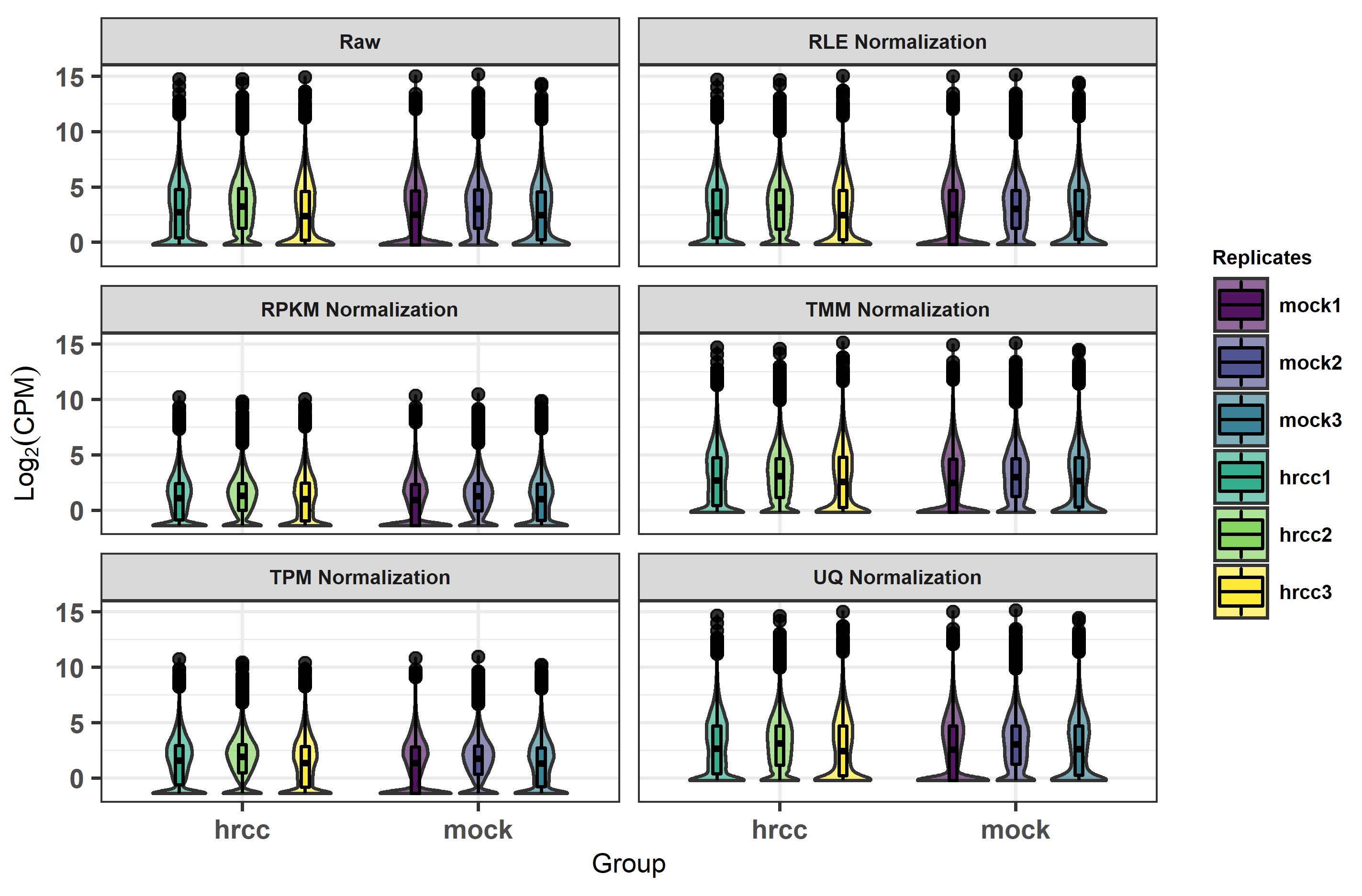
Figure 1. Box plot of normalization methods and raw expression log2 (CPM) outcomes.
We perform a PCA analysis to explore the performance of different batch effect removal methods (Figure 2). From the PCA analysis, we see that the clustering of samples is not ideal, as mock3 and hrcc3 are far from the other four samples, so we infer this is caused by batch effects. Figure 2C, D, E, and F show the PCA clustering results based on four batch effect removal methods (parametric ComBat, non-parametric ComBat, ComBat_seq, and SVA, respectively). In Figure 2C and D, the PC1 percentage shows a significant improvement, as two clusters clearly separate from each other (control group on the left, and hrcc group on the right). Therefore, the batch effect removal procedure can reduce bias, and we suggest that researchers add it to their own research pipeline.
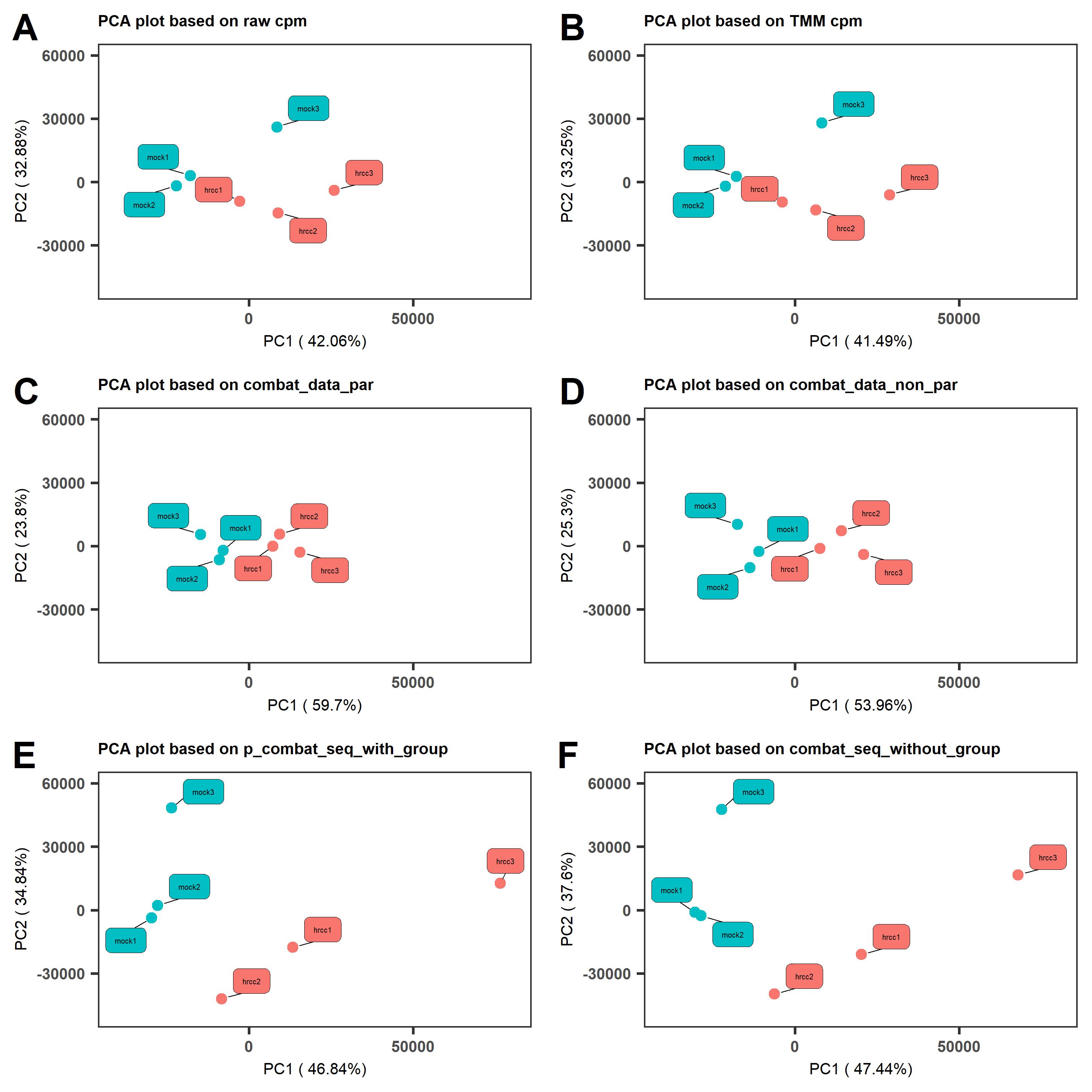
Figure 2. The plot of PC1 and PC2 based on different batch removal methods (C, D, E, and F) compared to raw CPM (A) and TMM normalized CPM (B).
Discussion
Normalization and batch effect removal are two necessary procedures in the analysis of gene expression. This protocol provides codes of commonly used R packages to perform normalization (TMM, UQ, RLE, RPKM, and TPM) and batch effect removal procedures (parametric ComBat, non-parametric ComBat, ComBat_seq, and SVA), based on raw count data. Readers can use the code in the protocol to learn the normalization and batch effect removal steps in detail. The output results, based on the example dataset, are also provided, so that readers can check their results against the given outputs. Due to space limitation, this paper only shows how to perform normalization and batch effect removal procedures based on R packages edgeR and sva, but we should note that many other packages can implement normalization (such as DESeq2 and limma) and batch effect removal (e.g., bapred). This paper does not include the comparison between different normalization and batch effect removal methods, because results are determined by input raw count datasets, and the experimental design continuously changes. Therefore, we suggest that researchers try different normalization and batch effect removal methods, and choose the most suitable ones.
Acknowledgments
This protocol was derived from the research in Dr. Zhenyu Jia’s lab, UC Riverside. The authors thank Dr. Zhenyu Jia for his review of the manuscript and helpful comments.
Competing interests
The authors declare that there are no conflicts of interest or competing interests.
References
- Anders, S. and Huber, W. (2010). Differential expression analysis for sequence count data. Genome Biol 11(10): R106.
- Abbas-Aghababazadeh, F. and Li, Q. (2018). Comparison of normalization approaches for gene expression studies completed with high-throughput sequencing. PloS one 13(10): e0206312.
- Bullard, J. H., Purdom, E., Hansen, K. D. and Dudoit, S. (2010). Evaluation of statistical methods for normalization and differential expression in mRNA-Seq experiments. BMC Bioinformatics 11: 94.
- Cumbie, J. S., Kimbrel, J. A., Di, Y., Schafer, D. W., Wilhelm, L. J., Fox, S. E., Sullivan, C. M., Curzon, A. D., Carrington, J. C., Mockler, T. C., et al. (2011). GENE-counter: a computational pipeline for the analysis of RNA-Seq data for gene expression differences. PLoS One 6(10): e25279.
- Johnson, W. E., Li, C. and Rabinovic, A. (2007). Adjusting batch effects in microarray expression data using empirical Bayes methods. Biostatistics 8(1): 118-127.
- Li, B., Ruotti, V., Stewart, R. M., Thomson, J. A. and Dewey, C. N. (2010). RNA-Seq gene expression estimation with read mapping uncertainty. Bioinformatics 26(4): 493-500.
- Leek, J. T., Scharpf, R. B., Bravo, H. C., Simcha, D., Langmead, B., Johnson, W. E., Geman, D., Baggerly, K. and Irizarry, R. A. (2010). Tackling the widespread and critical impact of batch effects in high-throughput data. Nat Rev Genet 11(10): 733-739.
- Leek, J. T. (2014). svaseq: removing batch effects and other unwanted noise from sequencing data. Nucleic Acids Res 42(21).
- Leek, J. T., Johnson, W. E., Parker H. S., Jaffe A. E. and Storey, J. D. (2014). sva: Surrogate Variable Analysis R package version 3.10. 0. DOI 10, B9.
- Love, M. I., Huber, W. and Anders, S. (2014). Moderated estimation of fold change and dispersion for RNA-seq data with DESeq2. Genome Biol 15(12): 550.
- McCarthy, D. J., Chen, Y. and Smyth, G. K. (2012). Differential expression analysis of multifactor RNA-Seq experiments with respect to biological variation. Nucleic Acids Res 40(10): 4288-4297.
- Robinson, M. D., McCarthy, D. J. and Smyth, G. K. (2010). edgeR: a Bioconductor package for differential expression analysis of digital gene expression data. Bioinformatics 26(1): 139-140.
- Robinson, M. D. and Oshlack, A. (2010). A scaling normalization method for differential expression analysis of RNA-seq data. Genome Biol 11(3): R25.
- Risso, D., Ngai, J., Speed, T. P. and Dudoit, S. (2014). Normalization of RNA-seq data using factor analysis of control genes or samples. Nat Biotechnol 32(9): 896-902.
- Ritchie, M. E., Phipson, B., Wu, D., Hu, Y., Law, C. W., Shi, W. and Smyth, G. K. (2015). limma powers differential expression analyses for RNA-sequencing and microarray studies. Nucleic Acids Res 43(7): e47.
- Trapnell, C., Williams, B. A., Pertea, G., Mortazavi, A., Kwan, G., van Baren, M. J., Salzberg, S. L., Wold, B. J. and Pachter, L. (2010). Transcript assembly and quantification by RNA-Seq reveals unannotated transcripts and isoform switching during cell differentiation. Nat Biotechnol 28(5): 511-515.
- Zhang, Y., Parmigiani, G. and Johnson, W. E. (2020). ComBat-seq: batch effect adjustment for RNA-seq count data. NAR Genom Bioinform 2(3): lqaa078.
Supplementary information
- Data and code availability: All data and code have been deposited to GitHub: https://github.com/Bio-protocol/Normalization-and-Batch-Effect-Removal.git.
Category
Plant Science > Plant molecular biology
Molecular Biology > RNA > Transcription
Bioinformatics and Computational Biology
Do you have any questions about this protocol?
Post your question to gather feedback from the community. We will also invite the authors of this article to respond.