A Reproducible FIJI-Based Workflow for Quantitative Analysis of Cartilage Histomorphometry 

ABSTRACT:
Quantitative assessment of cartilage architecture is essential for understanding skeletal development, tissue homeostasis, and disease progression; however, standardized and accessible workflows for reproducible morphometric analysis remain limited. This paper outlines a reproducible protocol using FIJI (Fiji Is Just ImageJ) software to quantitatively measure cartilage properties from histological images of stained tissue sections.
The protocol enables the measurement of key parameters, including cartilage area and length, stain intensity (as a surrogate for matrix composition), zonal organisation (superficial, middle, and deep zones), zone-wise chondrocyte cell count and circularity, chondron enumeration, and lacunar area. All these measurements can be made in physical units, e.g. micrometers (µm), by first performing a scale calibration of the images before analysis. All analyses are performed using built-in FIJI functions, without the need for specialized plugins.
In this study, human fetal cartilage histological sections were used to demonstrate the analysis and outline the step-by-step workflow described in this protocol.
This protocol offers an open-source workflow for quantitative cartilage histomorphometry, applicable across diverse research contexts, including developmental biology, disease modelling, and the assessment of cartilage healing and regeneration following therapeutic or tissue engineering interventions.
Keywords: Quantitative comparison, Cartilage properties, FIJI, morphometry
BACKGROUND:
Cartilage properties vary significantly across the lifespan as the tissue transitions from a phase of rapid growth and matrix deposition to one of load-bearing function and eventual degeneration with age [1]. Fetal cartilage is typically more cellular with proliferative regions, whereas adult cartilage exhibits a well-defined zonal organization and reduced cellularity [2–3]. Quantitative assessment of these structural and compositional features requires accurate and reproducible morphometric analysis of histological cartilage sections.
FIJI is a widely used open-source image analysis platform commonly applied in histomorphometry studies. However, a standardized and reproducible workflow integrating multiple quantitative parameters such as cartilage length, cartilage area, stain intensity (as a surrogate of matrix composition), zonal organization, and cell count remains limited [4–8].
The development of a structured protocol for quantitative cartilage histomorphometry would enable consistent analysis across studies, facilitate reproducibility, and support applications in developmental biology, osteoarthritis research, and tissue engineering.
MATERIALS: 
A. BIOLOGICAL MATERIALS
Fetal cartilage samples were obtained from the knee of who had been spontaneously aborted or terminated due to medical reasons after obtaining written informed consent from the parents. The Institutional Review Board (Christian Medical College, Vellore) approved the research protocols for this study. All methods used ensured compliance with all relevant guidelines and regulations
B. REAGENTS
Safranin-O stain (for proteoglycan visualization)
Masson’s Trichrome staining kit (for collagen and matrix visualization)
Collagen type II primary antibody (for immunohistochemistry, if applicable)
Appropriate secondary antibody and detection reagents (for immunohistochemistry, if applicable)
C. IMAGE ACQUISITION
Brightfield microscope for histological imaging (e.g., Olympus/Leica)
Digital camera attached to microscope
Histological images acquired at defined magnifications (e.g., 10×, 20×) and saved in a lossless format (e.g., TIFF)
Life Technologies EVOS FL Auto Full Scan Imaging System and associated EVOS FL Auto software.
D: EQUIPMENT:
Computer Specifications:
1.    A 64-bit operating system that has Windows 7 or greater, Mac OS X 10.11 or greater, or Linux with kernel supporting GLIBC 2.14 and GLIBCXX 3.4.15 (typically kernels 2.6.39).
2.    Any computer with Java-based operating system and Excel available
SOFTWARE:
1.    Free ImageJ Fiji software (Schindelin J, Arganda-Carreras I, Frise E, Kaynig V, 
Longair M, Pietzsch T, Preibisch S, Rueden C, Saalfeld S, Schmid B, Tinevez JY, White DJ, Hartenstein V, Eliceiri K, Tomancak P, Cardona A, https://imagej.net/Fiji/Downloads), version 1.2 (no specific plugin was used)
STEP-BY-STEP FIJI WORKFLOW FOR QUANTIFICATION OF CARTILAGE HISTOLOGY
I.    HOW TO SET SCALE BAR
A)    Open Image
1.    Open FIJI
2.    Go to File > Open and select a reference image with known distance.
3.    Using the “straight-line selection tool” , draw a line over a feature in the image that corresponds to a known distance.
4.    Navigate to Analyze > Set Scale. A dialog box will appear. 
B)    Set Scale
In the Set Scale window:
•    Distance in Pixels - automatically filled based on the length of the line selection.
•    Known distance – enter the real value of scalebar (eg.100)
•    Unit of Measurement – type μm
•    Tick Global - if you want the same calibration for all images.
•    Click OK
 

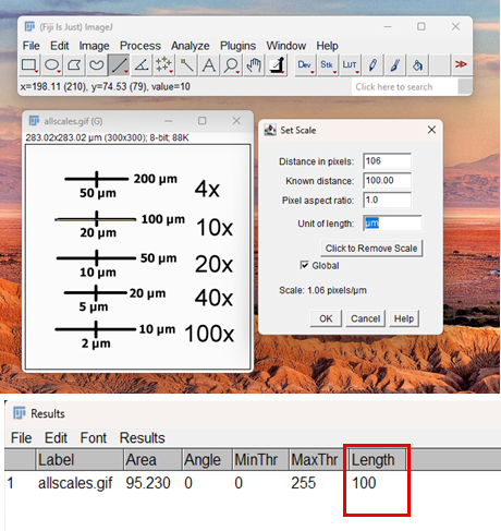
Fig. 1: Representative image with scale bar. The inset dialog box displays the calibration parameters (Scale: 1.00 pixels/µm) used for morphometric analysis.
5.    Now, to check if the calibration worked
•    Draw another line on the scalebar
•    Go to Analyze > Measure
6.    The result should show approximately 100 µm (or whatever your scale bar value is)
Note: Ensure the line exactly overlaps the scale bar to avoid calibration errors.

II.    HOW TO FIND THE CARTILAGE AREA
A)    Open Image
1.    Open FIJI
2.    Navigate to File > Open and select your desired image.
3.    To preserve the original data, create a duplicate of the image for analysis by clicking Image > Duplicate
B)    Set Scale
Define the spatial scale of the image as described in Section 1 ("HOW TO SET SCALE BAR"). This step is essential for obtaining area measurements in physical units such as micrometers (µm).
C)    Area Measurement
4.    Go to Image> Adjust> Colour Threshold
5.    Adjust the lower and upper sliders to select the pixel intensity range corresponding to your features of interest. The thresholded area will be highlighted in red by default.
6.    Select a thresholding method from the dropdown menu (e.g., Default, Otsu) for automatic thresholding, or manually adjust the sliders for interactive segmentation.

7.     Go to Process> Binary> Make Binary.

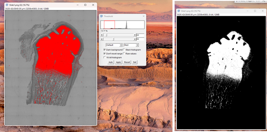
Fig. 2: Thresholding image for area measurement.

     8. Click the Freehand Selection Tool in the ImageJ toolbar. Manually trace the boundary of the specific zone to be analyzed.

     9. Go to Edit > Clear Outside. This deletes everything outside the traced selection.

    10. Go to Process> Binary> Fill holes. This is done to remove noise and artifacts from the image

D) Set Measurements

     11. Navigate to Analyze> Set measurements to define which parameters will be calculated and recorded during measurement.

     12. In the dialog box, check the following boxes:

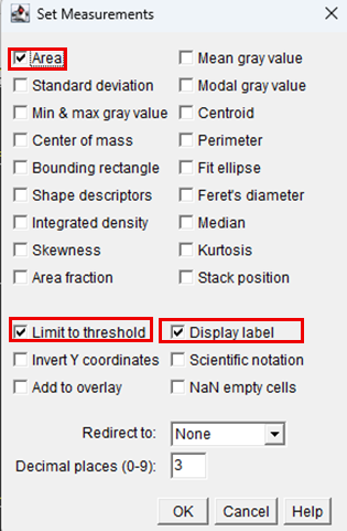
13.    After selecting the desired parameters, click OK.
14.    Click on Analyze > Measure
15.    A Results window will appear, displaying the measured area (and any other selected parameters) for the region of interest.
16.    Export the measurements from the Results table by selecting File > Save As for further statistical analysis.
 

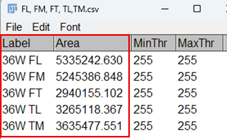
Fig. 3: Results obtained for measurement of area
 

Note: When image analysis is run on more than one image with the same Results window open, all further output of measurements will be added to the same Results window. If you close the old Results window first, then a new window will be opened with each analysis separately.

1. HOW TO MEASURE MEAN STAIN INTENSITY

   A. Open Image

   1. Open FIJI

   2. Navigate to File > Open and select your desired image.

   3. To preserve the original data, create a duplicate of the image for analysis by clicking Image > Duplicate

   B. Set Scale

Define the spatial scale of the image as described in Section 1 ("HOW TO SET SCALE BAR"). This step is essential for obtaining area measurements in physical units such as micrometers (µm).

         C. Mean Stain Intensity

               4. Image> Colour> Colour Deconvolution. In the dialog box, select the vector that matches your stained image, i.e., look for a                    similarly named vector in the list (such as the name of the stain or antibody used in your experiment). For example: use RGB                     for Safranin-O, H DAB vector for Collagen-II immunohistochemistry, and Masson Trichrome for Masson Trichrome sections. 

After selecting the appropriate vector, the software analyses each stained pixel of the image.  For each pixel, it calculates how much of the colour comes from each stain. These calculated amounts are then placed into separate output channels, so that each channel contains only one stain's signal. Consequently, the initial channel displays only the initial stain, the second channel displays only the second stain, and so forth, with little cross-contamination among channels. This enables specific visualization and quantification of each stain. 

For example, in an image stained with haematoxylin (blue‑purple) and DAB (brown), the H DAB vector instructs the software to separate the two colours. One resulting channel shows only haematoxylin, the other only with DAB, and a neutral background. This prevents the counterstain from interfering with measurements of DAB staining.

                  5. Clicking "OK" will generate a new image stack, typically with 2 or 3 channels,

each dividing the original stained image into an independent stain-specific components (e.g., haematoxylin alone, DAB alone). Identify the channel in which your target stain appears the strongest, and has minimal cross-contamination with other stains, and close the remaining ones.

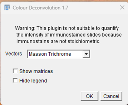
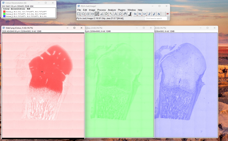
Fig. 4: Colour deconvolution of Masson Trichrome vector. This method isolates specific color components to enhance feature detection prior to quantification.

 

           6. Go to Image > Type> 8 bit to ensure uniform bit depth for intensity measurements.

           7. Go to Edit > Invert.

           8.Using the Freehand selection tool from the toolbar, manually trace around area where stain intensity is to be measured.

           9. Go to Analyze> Set measurements to define which parameters will be calculated and recorded during measurement.

           10. In the dialog box, check the following boxes:

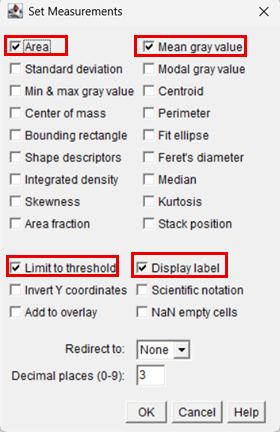
                 11. After selecting the desired parameters, click OK.

                 12. Click on Analyze > Measure

                 13. A Results window will appear, displaying the mean intensity for the region of interest.

                 14. Export the measurements by selecting File > Save As for further statistical analysis.

Note: When image analysis is run on more than one image with the same Results window open, all further output of measurements will be added to the same Results window. If you close the old Results window first, then a new window will be opened with each analysis separately.

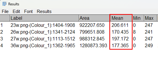
                                      Fig. 5: Results obtained for cartilage stain intensity
                   IV.    HOW TO MEASURE ZONAL DIVISION OF CARTILAGE
A)    Open Image
1.    Open FIJI
2.    Navigate to File > Open and select your desired image.
3.    To preserve the original data, create a duplicate of the image for analysis by clicking Image > Duplicate
B)    Set Scale
Define the spatial scale of the image as described in Section 1 ("HOW TO SET SCALE
BAR"). This step is essential for obtaining area measurements in physical units such as micrometers (µm).
C)    Defining zonal areas
Total cartilage length was measured from the articular surface to the osteochondral
interface using the straight-line tool. Zonal regions will be calculated based on the total
image height. Standardized zones were then defined as relative percentage depths:
superficial (upper 10%), middle (10–50%), and deep (50–90%).

4.    Go to Image > Show Info 
A meta window will open displaying file name (Slide1.png), image
dimensions (width × height), Bit depth (8-bit, 16-bit, RGB, etc.) pixel size / spatial
calibration (e.g., µm per pixel if the image is calibrated).
 

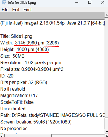
Fig. 6: The "Info" window provides key metadata for "Slide1.png", including physical width (3145.10 µm), height (4000 µm), pixel size (0.98 x 0.98 µm²), and resolution (1.02 pixels/µm).

 

5. Zonal Division of given area: 

i)    Creation of the Superficial Zone ROI (Upper 10%)
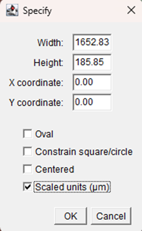
a.    Click Edit > Selection > Specify.
b.    In the dialog box, enter the following values:
o    Width: full image width (eg. here, 1652.83)
o    Height: 10% of the total image height
o    X: 0
o    Y: 0
c.    Click OK.
d.    In the ROI Manager, click Add to store the selection.
e.    Rename the ROI as Superficial Zone.
ii)    Creation of the Middle Zone ROI (10–50%)
a.    Select Edit > Selection > Specify again.
b.    Enter the following values:
o    Width: full image width (eg. here, 1652.83)
o    Height: 50% of the total image height
o    X: 0
o    Y: 10% of the total image height
c.    Click OK.
d.    Click Add in the ROI Manager.
e.    Rename the ROI as Middle Zone.
iii)    Creation of the Deep Zone ROI (50–40%)
a.    Select Edit > Selection > Specify.
b.    Enter the following values:
o    Width: full image width (eg. here, 1652.83)
o    Height: 90% of image width
o    X: 0
o    Y: 10% of total image height + 50% of the total image height
c.    Click OK.
d.    Click Add in the ROI Manager.
e.    Rename the ROI as Deep Zone.
f.    All three zonal ROIs will now be stored in the ROI Manager.
 

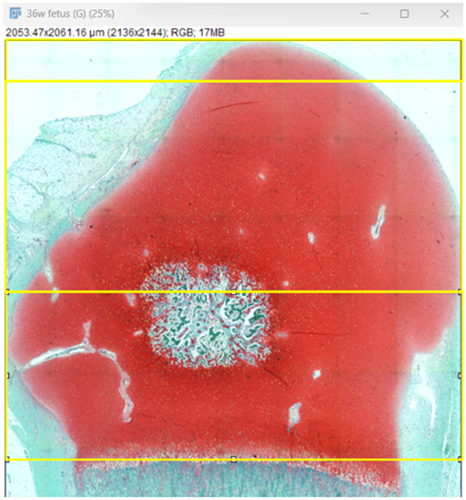
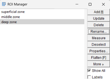
Fig. 7: Zonal division of cartilage- superficial (10%), middle (50%), 
and deep (90%).

D)    Zonal area measurement
5.    Select the desired ROI in the ROI Manager.
6.    To preserve the original data, create a duplicate of the image for analysis by clicking Image > Duplicate.
7.    Click OK.
8.    A new image containing only the selected zonal region will open.
9.    Repeat this process for the superficial, middle, and deep zones.
10.    Select the duplicated zonal image (superficial, middle, or deep zone) that will be analyzed.
11.    Navigate to Image> Colour> Colour Deconvolution. In the dialog box, select Masson Trichrome from the list of stain vectors. Click OK.
12.    Three separate channel images will be generated (Colour_1, Colour_2, Colour_3). Examine the three channels and select the channel in which the cells are most clearly visible within the ROI.
13.    Convert the selected channel to grayscale by selecting: Image > Type > 8-bit.
14.    To remove background areas outside the tissue, select the Freehand Selection Tool  from the toolbar. Carefully outline the tissue region that needs to be analyzed, excluding surrounding empty space or slide background.
15.    Once the tissue area is selected, navigate to: Edit > Clear Outside. This step removes all regions outside the selected tissue boundary, ensuring that only the cartilage tissue remains for analysis.
16.    Convert the image to a binary format by selecting: Process > Binary > Make Binary.
17.    To remove small gaps within detected objects and improve segmentation, select: Process > Binary > Fill Holes. This step fills internal gaps within segmented nuclei and improves particle detection.
18.     Apply thresholding to isolate nuclei: Image > Adjust > Threshold.
19.    Adjust the threshold sliders until the nuclei are distinctly highlighted while minimizing background noise. Click Apply to finalize the thresholded binary image.

20. Configure measurement settings by navigating to: Analyze > Set Measurements. Enable the following parameters:

21. After selecting the desired parameters, click OK.

22. Click on Analyze > Measure

23. A Results window will appear, displaying the measured area (and any other selected parameters) for the region of interest.

24. Export the measurements from the Results table by selecting File > Save As for further statistical analysis.
 

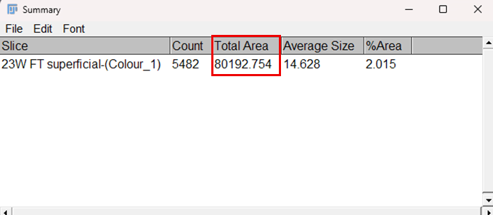
Fig.8: Results table for zone-wise area measurement

Note: ROI Manager for multiple sections of the same image– Open all segemented images of interest. Add ROIs into the ROI Manager (Analyze > Tools > ROI Manager) and click ‘Measure’. Results for every image will be appended to the same window.

V.    HOW TO PERFORM CELL COUNT AND CIRCULARITY:
A)    Open Image
1.    Open FIJI
2.    Navigate to File > Open and select your desired image.
3.    To preserve the original data, create a duplicate of the image for analysis by clicking Image > Duplicate
B)    Set Scale
Define the spatial scale of the image as described in Section 1 ("HOW TO SET SCALE BAR"). This step is essential for obtaining area measurements in physical units such as micrometers (µm).
C)    Cell count and circularity:
Steps 1–11 were performed as described in the zonal area measurement procedure to obtain individual zonal images and convert the selected colour channel to 8-bit grayscale.
4.     Measurement parameters were configured by navigating to Analyze > Set Measurements and enabling the following options:

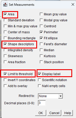
Selection of shape descriptors enables automatic calculation of cell circularity.
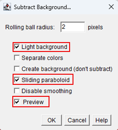
5.    Navigate to Process > Subtract Background.
6.    In the Subtract Background dialog box that appears:
•    Set an appropriate Rolling Ball Radius depending on image resolution.
•    Tick the options Light Background and Sliding Paraboloid.
7.    Click OK to apply background subtraction. This step reduces uneven illumination and improves contrast prior to further image processing and quantitative analysis:
 

8.    Thresholding was performed to isolate the chondrocyte nuclei by selecting Image > Adjust > Threshold.
9.    The threshold sliders were adjusted until the nuclei were clearly highlighted while minimizing background noise, after which Apply was selected to generate the thresholded binary image.
10.    To separate closely adjacent or touching objects, navigate to Process > Binary > Watershed.
11.    The Watershed function segments overlapping structures by creating boundaries between connected regions, enabling accurate identification and counting of individual objects.
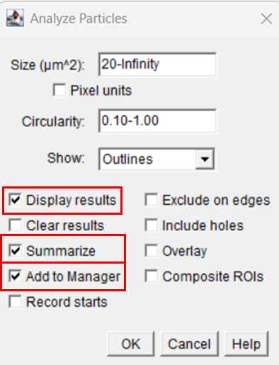
12.    Chondrocyte nuclei were quantified using Analyze > Analyze Particles.
13.    Particle analysis parameters were defined as follows:

14.    Upon execution, FIJI automatically detected and enumerated the nuclei within the defined ROI and recorded morphometric parameters for each particle.
15.    The Results window displayed measurements for each detected nucleus, including area, perimeter, and circularity values. The summary output provided the total cell count for each cartilage zone.
16.    All measurements were exported from the Results table for subsequent statistical analysis.
 

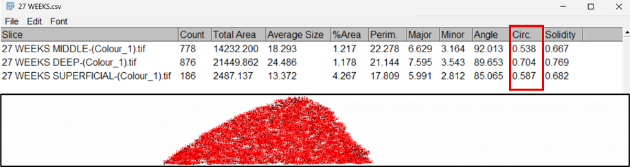
Fig.9: Results obtained for zone-wise cell count

Note: ROI Manager for multiple sections of the same image– Open all segemented images of interest. Add ROIs into the ROI Manager (Analyze > Tools > ROI Manager) and click ‘Measure’. Results for every image will be appended to the same window.