


Preparation of Moss Tissue for Cryo-Electron Tomography by High-Pressure Freezing, Focused Ion Beam Milling, and Lift-Out


发布: 2026年10月20日第16卷第20期 DOI: 10.21769/BioProtoc.5855 浏览次数: 15
评审: David PaulBeatrice LiWeidong An
 PDF
PDF  Q&A
Q&A
参见作者原研究论文
The authors used this protocol in:

May 2025





Abstract
Cryo-electron tomography (cryo-ET) is a powerful imaging technique that allows visualizing the molecular landscape within cells. In contrast to traditional preparations for electron microscopy deploying chemical fixation and contrasting agents, cryo-ET directly images cryo-fixed, i.e., vitrified samples, providing a faithful and near-native representation of cellular ultrastructure and its macromolecular constituents. While cryo-ET in combination with thinning by focused ion beam (FIB) milling is well established for single small or thin cells that can be vitrified by plunge freezing, its application to tissues is still challenging in terms of vitrification and thinning strategies. Intact plant tissues are particularly difficult, due to their relatively large cell size and the presence of vacuoles, which often occupy a large fraction of cells and usually do not vitrify. Here, we describe two methods for vitrification of the filamentous tissue (protonemata) of moss (Physcomitrium patens) by two high-pressure freezing (HPF) approaches. We also describe in detail how to prepare thin sections (lamellae) suitable for cryo-ET data acquisition by either on-grid FIB milling or lift-out with three different attachment methods that can be applied depending on skill and experimental setup of users. For the preparation of lift-out lamellae, we introduce an additional trimming step that can help to improve lamella quality. We illustrate how subcellular structures can be targeted by aiming for cell junctions using cryo-fluorescence light microscopy. The different preparation procedures can be used for samples of different sizes and other multicellular systems.
Key features
• This protocol builds on serial lift-out [1] but was adapted for moss and can be applied to other species and tissues, as described in [2].
• We describe two high-pressure freezing approaches for different specimen sizes and procedures for sample screening and targeted lamella preparation aided by cryo-fluorescence light microscopy.
• We describe on-grid lamella preparation and three lift-out approaches with a novel, more robust attachment mode.
• By applying an additional trimming step for lift-out sections, this protocol was optimized for lamella quality rather than quantity.
Keywords: High-pressure freezing (HPF) Cryo-fluorescence light microscopy
Cryo-focused ion beam milling (cryo-FIB)
Lift-out
Cryo-electron tomography (cryo-ET)
Physcomitrium patens
Cryo-correlative light and electron microscopy
Cryo-fluorescence light microscopy
Cryo-focused ion beam milling (cryo-FIB)
Lift-out
Cryo-electron tomography (cryo-ET)
Physcomitrium patens
Cryo-correlative light and electron microscopy
Graphical overview
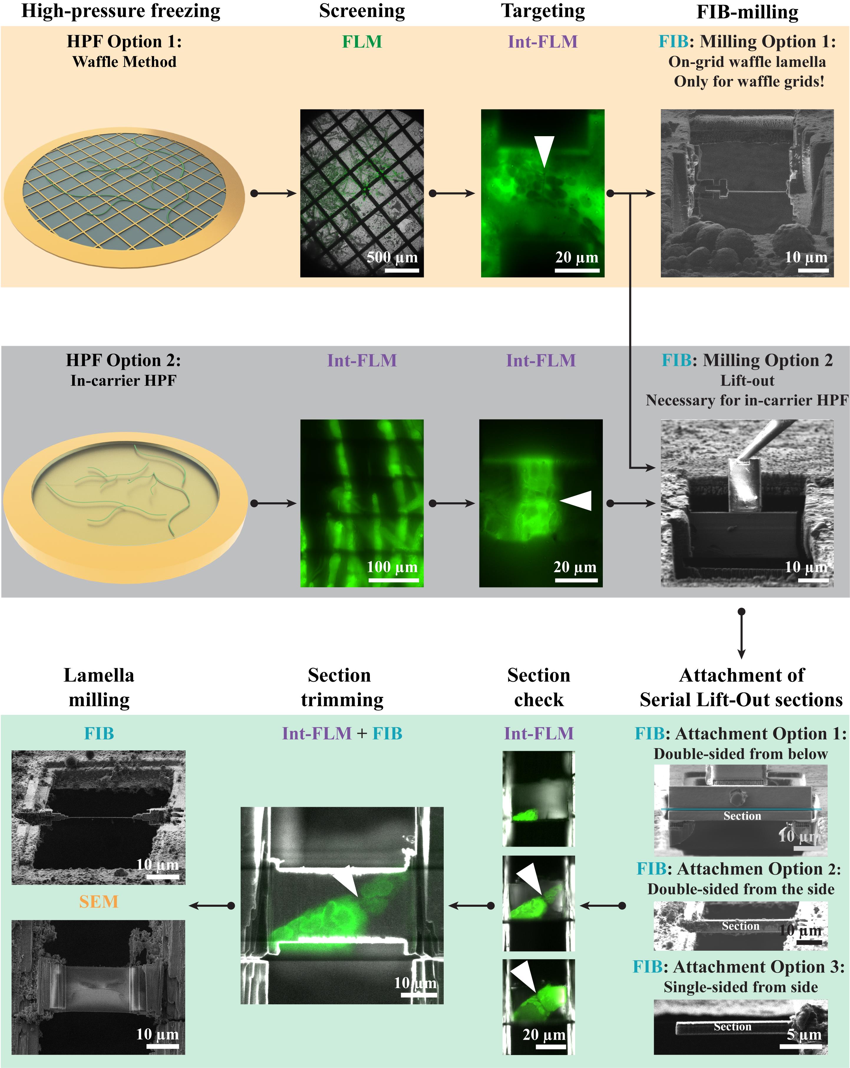
Overview of the protocol’s workflows. First, P. patens protonemata cells are high-pressure-frozen either by the waffle method or inside high-pressure freezing (HPF) carriers. Next, samples are screened in an external cryo-fluorescence light microscope (FLM) or an FLM integrated (int-FLM) into a cryo-focused ion beam (FIB) instrument. For waffle grids, on-grid lamella preparation is possible. To generate lamellae from in-carrier frozen samples, lift-out is required. Here, the serial lift-out approach is employed, in which the initial lift-out block is cut into several sections, which are attached to a receiver grid. Three distinct attachment modes are described: (1) double-sided attachment from below, (2) double-sided attachment from the side, and (3) single-sided attachment. Afterward, sections can be assessed for the presence of the target area and trimmed to remove excessive material before they are thinned to their final thickness in the lamella milling step.
Background
Cryo-electron tomography (cryo-ET) is a powerful method at the interface between structural biology and cell biology, which allows visualizing the molecular landscape within cells in 3D [3,4]. The first step in the workflow is cryo-fixation by vitrification, in which the sample is rapidly cooled to temperatures well below -150 °C while avoiding the formation of crystalline ice, i.e., transferring water into a vitreous state [5]. This step is critical because it arrests the cell in a frozen-hydrated, near-native state. Cells thinner than approximately 10 μm can often be vitrified by plunge-freezing. In this process, cells are applied as a thin film onto a grid for electron microscopy and plunged into a cryogen [6]. Cells thicker than a few hundred nanometers must then be thinned before they can be imaged in a transmission electron microscope (TEM). Here, cryo-focused ion beam (FIB) milling has become the method of choice in the field: a focused beam of Gallium ions is used to ablate material above and below an area of interest until only a sufficiently thin sheet of material remains that is still supported by the bulk sample on its sides [7]. These sheets are termed lamellae. To identify target areas within vitreous samples, cryo-correlative light and electron microscopy (CLEM) techniques have been developed, which correlate FIB and SEM images to images recorded in an external cryo-fluorescence light microscope (FLM) [8] or an FLM integrated (int-FLM) into the chamber of the FIB system [9]. The resulting lamellae are then imaged in a cryo-TEM. In cryo-ET, a set of TEM images is recorded in the same area from a defined range of angles. This data is used to computationally yield a 3D reconstruction of the pleomorphic environment of the cell, a volume referred to as a tomogram [10].
Many multicellular samples, however, are too thick to be vitrified by plunge-freezing. Especially, intact plant tissues are challenging due to their large size and the presence of vacuoles occupying large fractions of the cell, with the tendency not to vitrify. An alternative approach to achieve vitrification is high-pressure freezing (HPF) [11,12]. The specimen is sandwiched between metal carriers, and a pressure of approximately 2,000 bar is applied while the sample is cooled by a jet of liquid nitrogen. Under these conditions, samples with a thickness of up to 200–300 μm can potentially be vitrified. Working with HPF samples, however, is more challenging and time-consuming than working with plunge frozen samples. Throughput and success rate are lower, and the CLEM approaches required to target biological material are tedious and time-consuming.
In this protocol, we describe in detail how we adapt the waffle method [13] and use in-carrier high-pressure freezing for protonemata of the moss Physcomitrium patens, which are filaments of single, cylindrical cells with diameters of 15–30 μm [14]. We lay out how to use cryo-fluorescent light microscopy and cryo-FIB milling for targeted lamella preparation, either by on-grid milling or serial lift-out [1] with three different attachment methods. The presented sample and lamella preparation strategies have advantages and disadvantages, which are discussed in [2] and can be deployed for other specimens beyond plant tissues. We uncover several pitfalls and critical steps, as pointed out at the respective steps in the workflow. Thus, we anticipate that this protocol can be a valuable resource for labs getting started with cryo-ET on multicellular samples.
Materials and reagents
Biological materials
1. Protonemata of Physcomitrium patens (Hedw.) ecotype Gransden cultures (International Moss Stock Center, Freiburg, Germany) cultivated for two weeks
Reagents
Reagents for P. patens culture
1. Agar (Sigma, catalog number: A1296)
2. Boric acid (H3BO3) (Roth, catalog number: P010.1)
3. Calcium chloride (CaCl2), water-free (Roth, catalog number: A119.1)
4. Cobalt (II) chloride hexahydrate (CoCl2·6H2O) (Roth, catalog number: 7095.1)
5. Copper sulfate pentahydrate (CuSO4·5H2O) (Roth, catalog number: P024.1)
6. Di-ammonium tartrate (Roth, catalog number: 0487.2)
7. Iron (II) sulfate heptahydrate (FeSO4·7H2O) (Roth, catalog number: P015.1)
8. Lithium chloride (LiCl) (Roth, catalog number: 3739.1)
9. Magnesium sulfate heptahydrate (MgSO4·7H2O) (Roth, catalog number: 8283.2)
10. Manganese (II) chloride tetrahydrate (MnCl2·4H2O) (Roth, catalog number: 0276.1)
11. Potassium aluminum sulfate dodecahydrate [KAl(SO4)2·12H2O] (Roth, catalog number: P724.2)
12. Potassium bromide (KBr) (Alfa Aesar, catalog number: 12612)
13. Potassium dihydrogen phosphate (KH2PO4) (Roth, p.a., catalog number: 3904.2)
14. Potassium hydroxide (KOH) (Chem Lab NV, catalog number: CL02.1195.1000)
15. Potassium iodide (KI) (Alfa Aesar, catalog number: A12704)
16. Potassium nitrate (KNO3) (Roth, catalog number: 8001.1)
17. Sodium molybdate dihydrate (Na2MoO4·2H2O) (Roth, catalog number: 0274.1)
18. Sodium hydroxide (NaOH) (Merck, p.a., catalog number: 106482)
19. Zinc sulfate heptahydrate (ZnSO4·7H2O) (Roth, catalog number: 7316.1)
Reagents for high-pressure freezing
1. Cetyl palmitate, synthetic (Roth, catalog number: 9229.2)
2. Ficoll 400 (Sigma, catalog number: F4375)
3. Acetone (technical grade)
4. Bleach (household bleach), e.g., Dan Klorix
5. Diethyl ether (Merck, p.a., catalog number: 31690)
6. Ethanol (technical grade)
7. Liquid nitrogen
Solutions
1. Trace element solution (see Recipes)
2. Growth medium (see Recipes)
3. Agar growth medium (see Recipes)
4. Cleaning solution for HPF carriers (see Recipes)
5. Cetyl palmitate solution (see Recipes)
6. Freezing buffer (see Recipes)
Recipes
Note: If not specified otherwise, all solutions are prepared with double-distilled water (ddH2O).
1. Trace element solution
| Reagent | Quantity per 1 L |
|---|---|
| Boric acid | 614 mg |
| Copper sulfate pentahydrate | 55 mg |
| Potassium bromide | 28 mg |
| Potassium aluminum sulfate dodecahydrate | 110 mg |
| Manganese (II) chloride tetrahydrate | 389 mg |
| Sodium molybdate dihydrate | 25 mg |
| Zinc sulfate heptahydrate | 55 mg |
| Lithium chloride | 28 mg |
| Cobalt (II) chloride hexahydrate | 55 mg |
| Potassium iodide | 28 mg |
Fill up to 1 L with ddH2O and filter with a sterilized membrane (pore size = 0.22 μm).
2. Growth medium
| Reagent | Volume per 1 L |
| Solution A | 10 mL |
| Solution B | 10 mL |
| Solution C | 10 mL |
| Solution DK | 10 mL |
| Solution DF | 10 mL |
| Trace element solution | 1 mL |
| 1 M calcium chloride (autoclaved) | 1 mL |
Fill up to 1 L with ddH2O and autoclave it.
Solution A: 500 mM Di-Ammonium tartrate (autoclaved)
Solution B: 25 g/L Magnesium sulfate heptahydrate (autoclaved)
Solution C, 25 g/L potassium dihydrogen phosphate (autoclaved). Adjust the pH to 6.5 with potassium hydroxide.
Solution DK: 101 g/L potassium nitrate (autoclaved)
Solution DF: 1.25 g/L Iron (II) sulphate heptahydrate (autoclaved)
3. Agar growth medium
| Reagent | Final concentration | Quantity per 1 L |
|---|---|---|
| Growth medium | n/a | 1 L |
| Agar | 0.8% (m/V) | 8 g |
Autoclave before use.
4. Cleaning solution for HPF carriers
| Reagent | Final concentration | Volume |
|---|---|---|
| Commercial bleach | n/a | 3 mL |
| 10 M NaOH | n/a | 3 mL |
5. Cetyl palmitate solution
| Reagent | Final concentration | Quantity |
|---|---|---|
| Cetyl palmitate | 0.5% (m/v) | 250 mg |
| Diethyl ether | n/a | 50 mL |
6. Freezing buffer
| Reagent | Final concentration | Volume |
|---|---|---|
| 40% (m/v) Ficoll 400 solution | n/a | 1 mL |
| Growth medium | n/a | 1 mL |
Laboratory supplies
1. Cartridge with cutout for FIB milling, i.e., cryoFIB AutoGrid (Thermo Fisher Scientific, catalog number: 1205101)
2. Cartridge without cutout, i.e., C-Clip ring (Thermo Fisher Scientific, catalog number: 1036173)
3. Clip rings, i.e., C-Clip (Thermo Fisher Scientific, catalog number: 1036171)
4. Cellophane sheets (325P, 80 mm) (A.A Packaging LTD)
5. Filter paper, Whatman, Grade 1
6. Grids, copper 400 × 100 mesh (e.g., Graticules Optics, catalog number: 07D00917)
7. Grids, copper with continuous support film, 50 or 100 mesh (e.g., Graticules Optics, catalog number: 03D01050/100, 03D01100/100
8. Grids, copper, half-moon with 4 pins (Ted Pella Inc, catalog number: 10GC04)
9. HPF carriers type A, 3 mm, gold-plated copper (Leica Microsystems, catalog number: 16770152)
10. HPF carriers type B, 3 mm, gold-plated copper (Leica Microsystems, catalog number: 16770153)
11. HPF carriers type B, 6 mm, gold-plated copper (Leica Microsystems, catalog number: 16770182)
12. Sterile filter (pore size = 0.22 μm) (Sigma-Aldrich, catalog number: S2GPT05RE)
13. Sterile Petri dish (92 × 16 mm) (e.g., Sarstedt, catalog number: 82.1473.001)
14. Lint-free cloth wipes
15. Cryo grid boxes (Thermo Fisher Scientific, catalog number: 1084591)
Equipment
1. Cartridge tweezers (Thermo Fisher Scientific, catalog number: 943290997631)
2. Clipping base/station (Thermo Fisher Scientific)
3. Clipping tools (Thermo Fisher Scientific)
4. Cryo-focused ion beam and scanning electron microscope (FIB/SEM) instrument with rotatable stage and needle-based lift-out system, e.g., Scios, Aquilos or Aquilos2
5. EasyLift system (Thermo Fisher Scientific)
6. Cryo FIB/SEM shuttle with 45° pretilt (Thermo Fisher Scientific)
7. Cryo light fluorescence microscope, e.g., Leica TCS SP8 (Leica Microsystems), confocal laser scanning microscope, two hybrid detectors
8. Cryo light fluorescence microscope objective, 50× air objective (Leica, catalog number: 506520), NA 0.9
9. EasyLift system (Thermo Fisher Scientific)
10. Grid box opening tool (Thermo Fisher Scientific)
11. Grid box storage system
12. Growth chamber (Binder KBW 400, catalog number: 9020-0339)
13. High-pressure freezer, e.g., Leica EM ICE (Leica Microsystems, catalog number: 16771801)
14. HPF sample holder half cylinder for 3 mm carriers (Leica Microsystems, catalog number: 16771849)
15. HPF sample holder half cylinder for 6 mm carriers (Leica Microsystems, catalog number: 16771847)
16. HPF sample holder middle plates for 3 mm carriers (Leica Microsystems, catalog number: 16771833)
17. HPF sample holder middle plates for 6 mm carriers (Leica Microsystems, catalog number: 16771834)
18. Integrated fluorescence light microscope, METEOR (Delmic), preferably with low NA/high working distance objective for FIB-view imaging
19. Integrated fluorescence light microscope objective [e.g., LMPLFLN 50× air objective (Olympus), NA 0.5, working distance = 10.6 mm]
20. Large and intermediate size tweezers, for handling of grid boxes, sample carriers, and sample holders in cryo and at RT
21. Homogenize/Disperser, Miccra MiniBatch D-9
22. DS-20/PG-SMIR rod
23. Laminar flow bench
24. Microwave
25. Water purification system, e.g., Milli-Q® system
Software and datasets
1. LAS X (Version 3.5.5.19976, Leica Microsystems, Wetzlar, Germany)
2. Odemis (Version 3.5.2, Delmic, Delft, Netherlands)
3. FIB/SEM user interface (Microscope Version 7.7.1 or higher, Thermo Fisher Scientific)
Procedure
This protocol describes two options for HPF of P. patens protonemata: (1) a modified version of the waffle method [13] adapted from [1] and (2) in-carrier high-pressure freezing. For users with on-grid milling experience, working with waffle grids may be easier than with HPF carriers. Freezing samples in HPF carriers potentially allows vitrifying larger samples and avoiding sample damage due to compression, but to obtain lamellae, the technically more demanding lift-out is required.
In order to prepare lamellae for cryo-ET data acquisition, on-grid waffle lamella milling and serial lift-out are presented. On-grid waffle lamella milling is only possible on waffle grids and does not require a lift-out system, but results in a single lamella per target area. In contrast, serial lift-out allows for more complete volume sampling as serial sectioning produces multiple lamellae per target area. For the attachment of serial lift-out sections, three methods are described: (1) double-sided attachment from below, (2) double-sided attachment from the side, and (3) single-sided attachment. The single-sided attachment requires the least precision but results in unstable lamellae. The double-sided attachment from the side needs the most precision but is the best compromise between stability and throughput. For the double-sided attachment from below, additional grid preparation steps are necessary, but the subsequent attachment is straightforward, resulting in the most stable lamellae. A more comprehensive discussion of advantages and disadvantages can be found in [2].
The protocol is specifically aimed at junctions between P. patens cells. These cell junctions are small, compared with the whole cell, and employing an integrated-fluorescence light microscope (int-FLM) for targeted trench milling is convenient. The targeting approach, however, can be used for any cellular structure that can be discerned in int-FLM images, e.g., by the expression of fluorescent fusion marker proteins.
Part I. The waffle workflow
A. Growing Physcomitrium patens protonemata
Note: Culture P. patens protonemata as described in [15], as follows:
1. Autoclave the agar growth medium (see Recipes) and cellophane sheets.
2. Melt the agar growth medium by heating it in a microwave if it is not liquid anymore.
3. In a laminar flow bench, plate 40 mL of the still liquified agar growth medium onto a sterile Petri dish.
4. After the agar growth medium is solidified, let it moisturize for 5 min, add an autoclaved cellophane sheet on top, and streak out air bubbles underneath with sterile, flat tweezers.
5. Harvest moss tissue from a 2-week-old plate (~1 g of wet yield per plate) and add to a 50 mL Falcon tube filled with 20 mL of ddH2O.
6. Homogenize the tissue with the disperser rod (3 × 3 s pulses on the lowest speed setting).
7. Spread 1 mL of homogenized P. patens liquid culture on a freshly prepared, cellophane-overlayed plate.
8. Grow P. patens for 2 weeks in a growth chamber at 25 °C with an 18/6 h light/dark cycle.
B. Waffle freezing, adopted from [1]
1. Clean 6-mm type-B HPF carriers (with one 300-μm cavity and one flat side) the day before freezing.
a. Incubate carriers overnight in a 15 mL Falcon tube with cleaning solution.
b. Wash carriers 3× with ddH2O and 3× with acetone.
c. Dry carriers on a filter paper.
2. Coat carriers with cetyl palmitate.
Note: Work under a fume hood.
a. Dip clean type-B carriers, one at a time, with tweezers into the cetyl palmitate solution.
b. Remove excess liquid by shaking it off and pushing the side of the carriers against filter paper.
3. Dry carriers on filter paper with the flat side facing up.
Critical: There should be a slight haze on the carrier, only obvious under the binoculars. If the layer is visible to the naked eye, the layer is likely too thick.
4. Prepare the Leica EM ICE high-pressure freezer and test the system.
a. Cool down the high-pressure freezer and the sample container.
b. Insert the sample container and wait for the system status to change to ready.
c. Freeze two samples with only the two half cylinders and a middle plate assembled without HPF carriers.
Note: This allows the system parts to equilibrate and adjust to the working temperature. It will also report the freezing curves, allowing to assess the normal working state of the machine. The pressure should persist at slightly above 2,000 bar for at least 250 ms and not longer than 450 ms. If that is not the case, contact Leica support.
5. Place a clean and coated type-B HPF carrier on a filter paper with the flat side facing up.
6. Add a 3 μL droplet of freezing buffer on the flat side of the carrier.
7. Place an EM grid with the continuous support film side facing down on the droplet.
Critical: The sample will be added on the “back” of the grid, i.e., the grid bar side, by filling it into the wells formed by the grid bars and the support film. For plunge-freezing, the sample is applied on the other side onto the film.
8. Remove excess buffer with a 0.5 × 2 cm piece of filter paper until the grid is lying flat on the carrier.
Critical: Initially, there will be convex cushions of buffer formed between the carrier and the support film. Blot until these cushions collapse and the support film contacts the carrier surface. This can be observed using the binoculars.
9. Add 3 μL of freezing buffer onto the grid and distribute it with the pipette tip or tweezers until the whole grid surface is covered.
10. Remove air bubbles by poking them with sharp tweezers. Alternatively, use slightly open tweezers and let the bubbles float into the liquid that is lifted between the tweezer legs by capillary force.
Critical: Air bubbles in the sample will be compressed upon high-pressure freezing and affect local pressure buildup negatively. They also expand again when the freezing chamber is depressurized and induce cracks in the sample, compromising subsequent steps.
11. Pick up a small patch of a protonemata from a plate and place it in the center of the grid.
Critical: Try not to squeeze the tissue with tweezers. This will damage the cells. Lift the tissue with the tip of a single leg of the tweezers to avoid squeezing.
12. If new air bubbles were created during the transfer of the tissue, remove them.
13. Place a second coated type-B carrier with the flat side down on top of the sample and press the sandwich lightly.
14. Remove excess buffer with filter paper around the carrier sandwich.
15. Place the sandwich in the middle plate on the lower plastic half cylinder.
16. Turn your tweezers upside down and press the sandwich thoroughly for 10 s with the reverse tweezer end.
Note: Pressing with the reverse tweezer end avoids damage to the tweezer tips or the carrier.
17. Immediately close the sample holder lid and freeze the sample.
18. After all grids are high-pressure-frozen, recover the grids by separating them from the carriers.
a. Remove all half-cylinders.
b. Remove middle plates and carriers that fell apart and have no grid attached to them.
c. If the sandwich is still in the middle plate, place it over a sufficiently large cavity (e.g., grid box holder) and push with blunt tweezers.
d. Collect all carriers with grids attached to them.
e. Place single carriers into, e.g., a grid box holder against the side wall
f. Use sharp tweezers to press at the 3, 6, 9, and 12 o’clock positions to break the continuous ice layer on the carrier.
g. Push the grid to the side, exerting 50% of the force in the lateral direction and 50% in the downward direction.
19. Mount the grids in cartridges with a cutout for FIB milling.
a. Before clipping, apply a red mark on the top of the cartridge in the 6 o’clock position opposite to the cutout and two blue markers in the 3 and 9 o’clock positions.
Note: This will help to align the grid when loading it into microscopes.
b. Clip the grid into the marked cartridge with the support film facing the clip ring.
Critical: In the waffle method, the sample is applied to the “back” of the grid on the opposite side of the support film. During clipping, the side with the support film must face the clip ring and the sample-containing side cartridge. This assures that the sample side is facing up when loading the grid into the microscope.
Pause point: Store grids in grid boxes at liquid nitrogen temperatures until use.
C. Sample screening in cryo-fluorescence light microscopy
1. Prepare the light microscope (e.g., Leica TCS SP8) by cooling it down, starting the lasers, and letting the system equilibrate for 30–60 min with the objective roughly at the height used for data acquisition.
2. Load a clipped waffle grid.
3. Focus on the sample and adjust the imaging parameters on some P. patens cells by recording reflected light (excitation: 488 nm; emission filter: 483–493 nm or no emission filter), cellular autofluorescence (excitation: 488 nm; emission filter: 500–750 nm), and transmitted light.
Note: The transmitted light and the autofluorescence of P. patens protonemata are sufficient to identify junctions between cells. For this target, no additional fluorescent marker is needed.
Critical: Keep the laser power as low as possible while still being able to identify your target area. Too-high laser power can devitrify your sample. The highest laser power that is safe to use depends on the system. With our setup, laser powers between 1% and 5% produced good results.
Critical: Adjust laser power and detector gain not to overload the HyD detectors. The most adequate imaging settings are dependent on the sample thickness.
4. Record a grid map (Figure 1A; spiral scan, tile image size = 512 × 512, pin hole size = 600 μm, pixel size = 580 nm).
Note: The pinhole can be fully open for this step, to collect as much fluorescence signal as possible—also from the layers above and below the focal plane.
5. Identify the location of grid squares containing target areas; in our case, single layers of undamaged P. patens protonemata with cell junctions at a distance of at least 50 μm from grid bars (Figure 1B).
Note: The distance to the grid bars is necessary to allow for on-grid lamella preparation. Furthermore, if those cells are partially on top of grid bars, they likely were damaged during high-pressure freezing and should be avoided.
Critical: Avoid grid squares with multiple cell layers. P. patens protonemata have a diameter of 15–25 μm, while the grid bars of typical EM grids are about 25 μm high. Multiple cell layers do not fit into the wells formed by the grid bars. Hence, multiple cell layers were likely squeezed and damaged by mechanical stress during high-pressure freezing (Figure 1C).
Critical: For on-grid lamella preparation, target areas should be located within ~800 μm from the center of the grid to assure that they are within the range of the TEM stage for cryo-ET data acquisition.
6. (Optional) Acquire z-stacks of the target area containing grid squares (Figure 1B; z-step size ≤ 1 μm encompassing the whole sample thickness, image size 2,048 × 2,048 pixels, pin hole size = 125 μm, pixel size = 140 nm).
Pause point: Unload the grid and store it in grid boxes at liquid nitrogen temperatures until use.
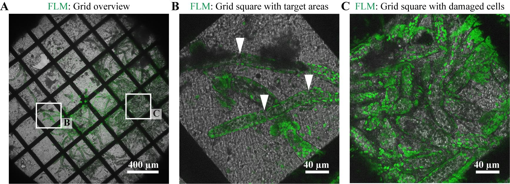
Figure 1. Sample screening in a cryo-fluorescence light microscope (FLM). Shown are the transmitted light (gray) and cellular autofluorescence (green) images of P. patens cells. (A) Overview of a P. patens protonemata waffle grid (75 mesh). (B) Grid square containing intact protonemata with cell junctions (white arrowheads) in the center of the square. (C) Grid square packed with multiple layers of protonemata. This tissue was likely mechanically damaged during high-pressure freezing (HPF) due to cell compression.
D. Trench milling in a dual focused ion beam and scanning electron microscope (FIB/SEM) with lateral targeting guided by an integrated–fluorescence light microscope (int-FLM)
Note: Lateral targeting and trench milling are performed in trench milling orientation (stage tilt = 7°, relative rotation = 180°; Figure 2). In this stage orientation, the optical axis of FIB and int-FLM are normal to the sample surface. Hence, FIB and int-FLM record sample top views.
Critical: The stage orientation angles and milling patterns described are only correct for the standard Thermo-Fisher Scientific FIB/SEM geometry (Figure 2): a shuttle with a 45° pretilt and the FIB/SEM scan rotation set to 180°.
Critical: Activate the drift suppression function of the FIB/SEM instrument during all trench milling steps. Activate at the lowest scanning electron microscope (SEM) magnification and drag the green targeting cross to the region that is to be milled.
1. Load a grid containing squares with target areas accessible to FIB milling into a FIB/SEM instrument equipped with int-FLM.
2. Move the stage into the lamella milling orientation (stage tilt = 20°, relative rotation = 0°; Figure 2).
3. Find the coincidence point of FIB and SEM roughly in the center of the grid and take a FIB and SEM image.
Note: FIB imaging settings: U = 30 kV, I = 1.5–10 pA; SEM imaging settings: U = 3 kV, I = 13 pA. Use the Everhart–Thornley detector (ETD) for detection.
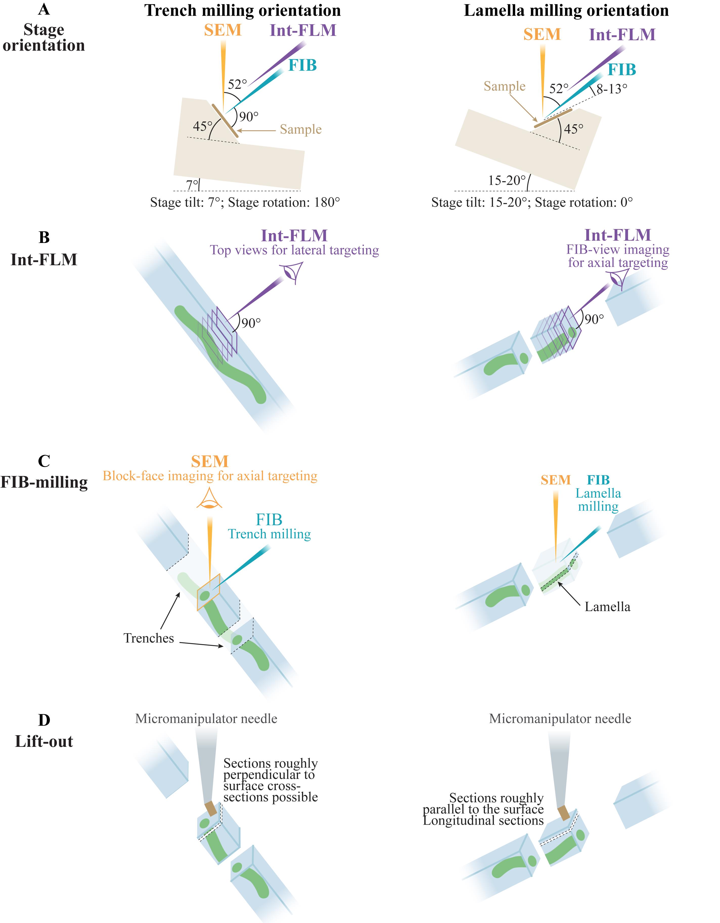
Figure 2. Scheme of the different stage orientations and their impact on imaging and lift-out steps. The left and right columns illustrate the trench milling and lamella milling orientation, respectively, which mainly differ with respect to a stage rotation of 180°. The angles apply to the geometry in FIB/SEM instruments produced by Thermo Fisher Scientific using a shuttle with 45° pretilt. (A) The shuttle with respect to stage tilt, stage rotation, and the relative angles of the FIB, SEM, and int-FLM optical axes. (B) Imaging planes of the int-FLM with respect to the sample in both stage orientations. In trench milling orientation (left), the int-FLM imaging plane corresponds to the grid plane and is used for lateral targeting, recording sample top views. In lamella milling orientation (right), the int-FLM images a plane close to the transverse section of the grid plane and may be used for axial targeting (“FIB-view” mode). (C) Imaging planes of the SEM and FIB modes. In trench milling orientation (left), the ion beam is normal to the sample surface and is used to mill trenches to the side of the target area. In lamella milling orientation (right), the ion beam is used to obtain thin lamellae from a shallow angle. (D) The orientation of the lift-out system in relation to the sample. In trench milling orientation (left), lift-out results in sectioning planes transverse to the sample surface and can yield cross-sections of protonemata. In lamella milling orientation (right), lift-out will yield sectioning planes at shallow angles toward the sample surface, resulting in longitudinal sections of protonemata.
4. Clear ice contamination with the FIB.
Critical: Do this before sputtering or applying a layer of metal-organic platinum with the gas injection system (GIS), as this will fix the contamination to the grid surface.
Note: A fine paint brush cooled to liquid nitrogen temperature can be used before loading the grid into the FIB/SEM system to remove vast amounts of frost on the front and/or back side of the grid.
a. Set to the lowest FIB magnification at an ion current (I) of 1 nA (dwell time = 50 ns, no line integration).
b. Activate the selected area window (hotkey F7) and adjust its size to about 100 × 100 μm.
c. Start scanning and rapidly move the selected area window over the grid from left to right and front to back while placing it on contaminated areas. You should see the contamination “hop” away (Figure 3).
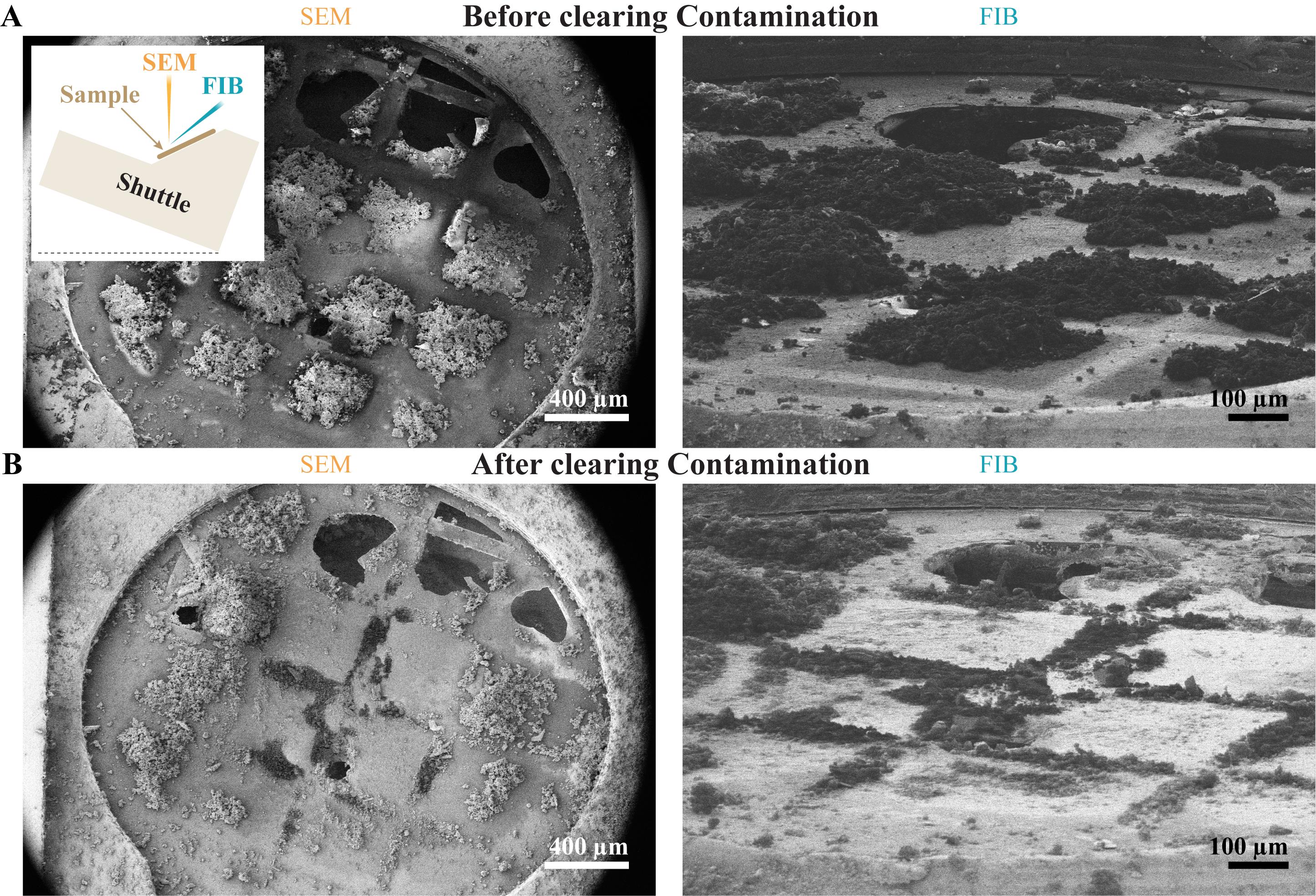
Figure 3. Clearing of contamination using the FIB. (A) Heavily contaminated waffle grid. The inset illustrates the location of the sample in the 45° pretilt shuttle with respect to the imaging direction of FIB and SEM. (B) After scanning at 1 nA with the selected area window over the grid surface, most of the ice is removed from the grid squares.
5. (Optional) Sputter coat the grid (p = 0.1 mbar, U = 1 kV, I = 10–30 mA, t = 15–30 s).
Note: The resulting platinum layer mitigates charging for thicker samples, resulting in higher quality of FIB and SEM images and more precise trench milling without drift suppression activated.
6. Rotate the stage to trench milling orientation (tilt = 7°, relative rotation = 180°; Figure 2).
7. Apply a layer of metal-organic platinum with the gas injection system (GIS) by moving the stage in trench milling orientation to the GIS working distance, inserting the GIS needle, and opening the GIS valve for 40 s (layer thickness ~200 nm on our systems).
Note: The GIS working distance and the thickness of the deposited layer of metal-organic platinum may vary between different FIB/SEM instruments. A calibration curve for your own instrument can be generated to estimate the thickness of the deposited layer, depending on valve opening times (see also General note 6).
8. Find the coincidence point on a grid square containing a target area as identified in the FLM before.
Note: The nearly featureless surface of waffle grids makes the correlation of external FLM and FIB images difficult. Thus, the int-FLM is convenient for targeted FIB milling. Yet, you should be able to estimate roughly where your target area is located within the grid square by FLM.
9. Mill a marker at a distance of 10–40 μm from your target area (cross-section, I = 3 nA, z = 0.5 μm).
Note: An asymmetric marker can be beneficial if FIB and int-FLM images are rotated with respect to one another; for example, an 8 × 8 μm square with a 6 × 16 μm rectangle aligned with their lower edges at a distance of 8 μm (Figure 4A).
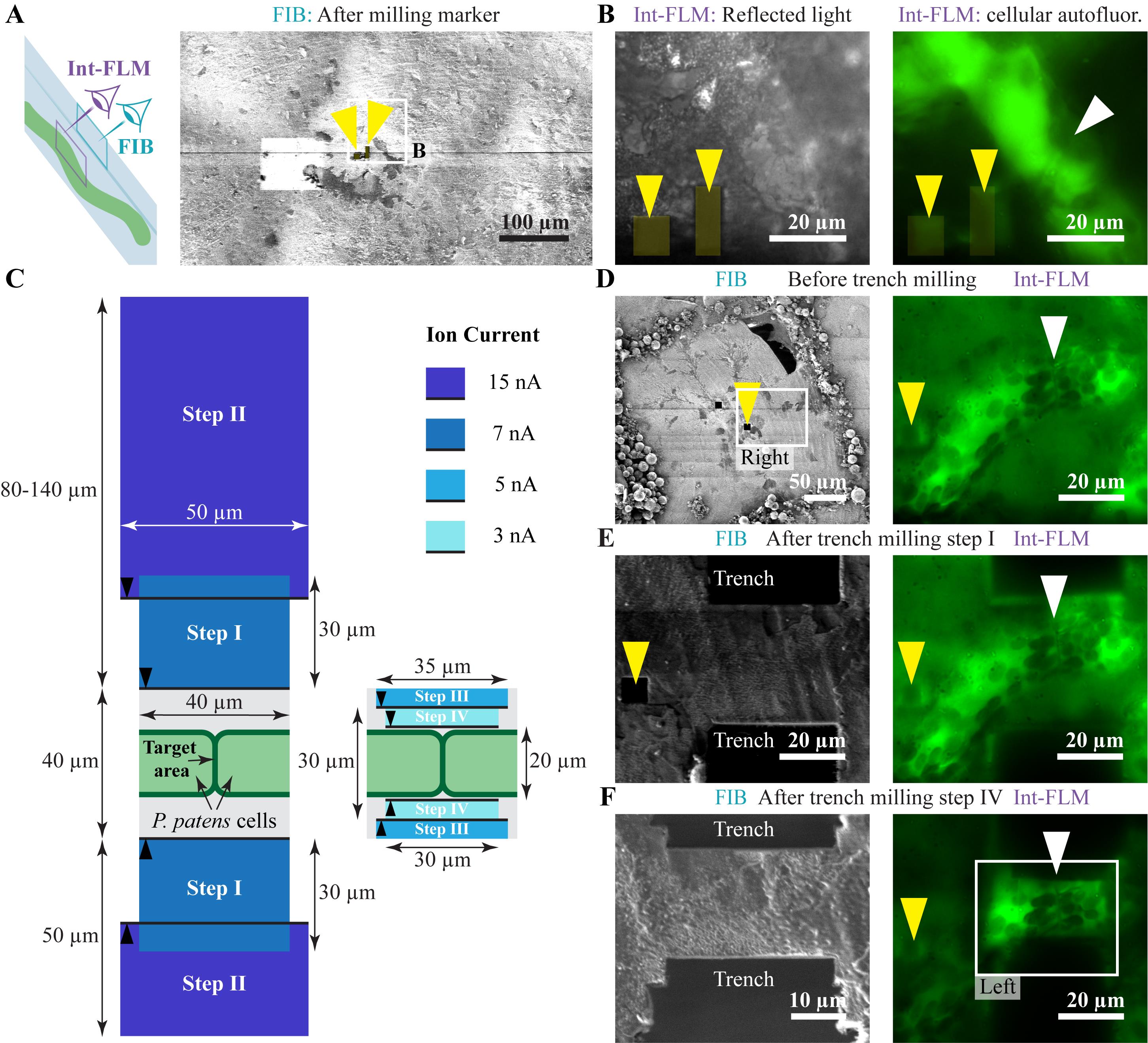
Figure 4. Lateral targeting and trench milling guided by the integrated fluorescence light microscope (int-FLM). (A) Sample top-view image recorded with the FIB. The asymmetric marker pattern is marked by yellow arrowheads. The scheme on the left illustrates the location of the sample with respect to the imaging direction of FIB and int-FLM. (B) Top views recorded with the int-FLM. The left panel shows the reflected light channel with marker holes, and the right panel shows the cellular autofluorescence revealing a cell junction. (C) Scheme of the trench milling patterns (only valid for FIB scan rotation of 180°). Black arrowheads indicate the milling direction. (D–F) FIB and int-FLM (cellular autofluorescence) top-view images of successive trench milling steps. Recording int-FLM images after each trench milling step is necessary to precisely center the target area. Marker holes and target areas are indicated by yellow and white arrowheads, respectively. The FIB milling patterns are provided in the Supplementary Information.
10. Use the int-FLM to record sample top views.
a. With the stage in trench milling orientation, focus the int-FLM on the sample surface and locate the marker pattern (Figure 4B).
Note: This is easiest accomplished using reflected light (excitation: 470 nm ± 10 nm; no emission filter).
b. Use the int-FLM to identify the target area nearby. For P. patens cell junctions, use cellular autofluorescence (excitation: 470 nm ± 10 nm; emission filter: 515 nm ± 15 nm; Figure 4B).
Critical: Keep the laser power as low as possible while still being able to identify your target area. Too-high laser power may devitrify your sample.
c. Determine the location of the target area with respect to the marker pattern. Measure the exact distance in the Odemis software.
Note: If the marker and target area are not within the same field-of-view in the int-FLM, consider milling another marker closer to the target area.
d. (Optional) Record z-stacks of the target area using the int-FLM (pixel size = 168 nm, 20–25 z-slices, z-step = 1 μm) to estimate the location of the target area within the thickness of the sample.
Notes:
1. For on-grid lamella preparation, we prefer target areas close to the top sample surface. It is substantially harder to prepare lamellae near the bottom surface, especially for thick samples.
2. If both FLM and int-FLM imaging are employed for targeting, the used excitation wavelengths and emission filters should ideally be the same for both imaging modalities. This assures the most reliable targeting. That is not the case here. Therefore, the fluorescence signals of FLM and int-FLM images (e.g., Figure 1 compared to Figure 4) appear different.
11. Use the relative location of the target area with respect to the marker pattern to define patterns for trench milling in the FIB user interface.
12. Mill trenches (holes) above and below the target area in trench milling orientation (Figure 4C).
Critical: Use regular cross-sections (Material: Si, Multipass: 4×) as they ablate material faster and generate smoother surfaces than rectangular patterns. The milling direction is always toward the target area.
Critical: Activate the drift suppression for every trench milling step. Before you change the ion current, deactivate the drift suppression, change the ion current, and activate drift suppression again.
Critical: If FIB-view imaging with the int-FLM is used for axial targeting (see section E), trench milling must be performed at a different stage tilt depending on the desired stage tilt for FIB-view imaging. For example, FIB-view imaging at a stage tilt of 20° requires trench milling at -6° in steps D12c–e.
a. FIB mill two horizontally aligned cross-sections with xyz-dimensions of 40 × 30 × 3 μm and a distance of 40 μm above and below the target area at 7 nA.
b. Vertically expand the trenches to 50 μm and 80–120 μm (z-dimension = 2.5 μm) below and above the target area, respectively, at 15 nA away from the target area.
Critical: The top trench should be as long as possible before it reaches a grid bar to be able to remove all the material below the lamella during thinning.
c. Reduce the size target area between the trenches in two steps to 35 × 30 μm (xy- dimension) at 5 nA (cross-section z = 2.5 μm).
Critical: If you want to use FIB-view imaging for targeting within the thickness of the sample (axial targeting), trench milling steps D12c–e must be performed at a different stage tilt (αTrench milling), dependent on the stage tilt you want to use for FIB (see section E).
αTrench milling = - αFIB-view + 14°
This is only correct for the standard Thermo Fisher Scientific FIB/SEM geometry and a shuttle with a pretilt of 45°.
Critical: In our hands, initial targeting is often imperfect. Record int-FLM images after each trench milling step and adjust the position of the patterns for the next step to improve positioning. This ensures that the target area is centered after trench milling (Figure 4D–F).
d. Reduce the size of the block between trenches 30 × 20 μm (xy-dimension) at 3 nA (cross-section z = 2.5 μm).
e. Polish the top front at 1 nA with a 1.5 × 30 × 3.5 μm cross-section (xyz-dimension). This face will be exposed to the ion beam during lamella milling and should be as smooth as possible (Figure 5A, B).
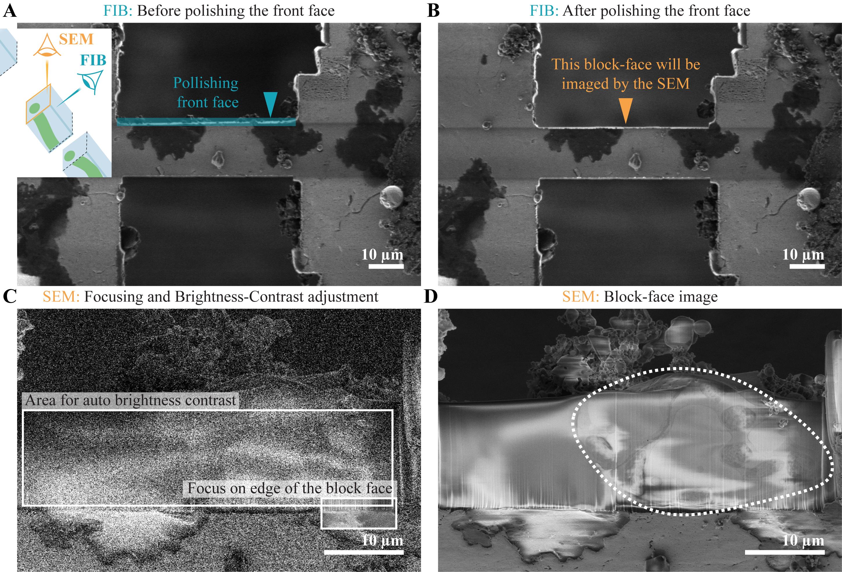
Figure 5. Axial targeting by SEM block face imaging. (A) FIB image after trench milling before polishing the front face. The blue rectangle indicates the milling pattern, and the blue arrowhead indicates the milling direction. The inset illustrates the sample surface after trench milling with respect to the imaging directions of SEM and FIB. (B) FIB image after polishing the front surface that will be imaged by the SEM. (C) Area for focusing and the auto brightness-contrast function prior to recording the SEM block-face image. (D) The resulting SEM block-face image. The tissue exposed at the surface is outlined by a dashed line.
E. Axial targeting
Note: Top views recorded with the int-FLM reliably localize the target area in the xy-plane of the grid. Due to the used widefield imaging system with low numerical aperture air objectives, however, the z-resolution is limited. Locating the target area in z (axial) is crucial to place the patterns for lamella milling and to assure that the target area is contained in the final lamella. Two methods can be employed for axial targeting.
1. Record a long-exposure SEM block face image after trench milling (Figure 5).
Note: Conduct SEM block face imaging with the stage in trench milling orientation (Figure 2). The top front of the block containing the target area is now exposed to the SEM. During fine milling, in lamella milling orientation, this front will be exposed to the FIB.
Critical: For lamella fine milling, the top front must be protected by a thick layer of metal-organic platinum. The image of the block face must be recorded before this layer is applied.
Critical: SEM block-face images can only be used for the rough axial targeting and only if cellular features are exposed at the top block face. Additionally, these features must generate sufficient contrast in SEM images. This is the case for, e.g., membrane structures and lipid bodies.
a. If not yet done, set the SEM acceleration voltage and current to 3 kV and 13 pA, respectively.
b. Center a spherical contamination next to the trenches in the SEM at the magnification used for block face imaging.
c. Focus on the contamination and correct astigmatism either manually or by running the Auto-stigmator function.
d. Center the block-face in the SEM field-of-view and focus on the edge between grid surface and block face (Figure 5C).
e. Create a selected area window (hotkey F7) on the block face and run the auto brightness-contrast function (hotkey F9) (Figure 5C).
f. Record a ~3,000 × 2,000 pixel image of the block face with a dwell time of 50 ns and 100 line integrations.
Note: The location of cells and organelles should be visible in the image (Figure 5D).
2. Record FIB-view images with the int-FLM.
Note: FIB-view images are recorded in lamella milling orientation from the same stage tilt at which lamella fine milling is performed. A more detailed description of FIB-view imaging can be found in (Capitanio et al.).
Critical: FIB-view imaging can only be performed with a high working-distance objective. If the working distance is below 10 mm, the objective may touch the shuttle before the sample is in focus. We use an Olympus LMPLFLN 50’ objective with a working distance of 10.6 mm.
Critical: For FIB-view imaging, the optical axis of the int-FLM should be normal to the front face after trench milling (Figure 6A, B). To achieve this, some trench milling (Figure 4C) are performed at a different stage tilt (steps D12c–e).
a. Rotate the stage into lamella milling orientation (Figure 2) and set the correct stage tilt (e.g., 20° if trench milling was performed at a stage tilt of -6°).
b. Use the reflected light channel to find the front of the trench.
c. Acquire int-FLM FIB-view images or z-stacks recording the reflected light (excitation: 470 nm ± 10 nm; no emission filter) and cellular autofluorescence (excitation: 470 nm ± 10 nm; emission filter: 515 nm ± 15 nm, pixel size = 168 nm, 20–25 z-slices, z-step = 1 μm). An overlay of FIB and FIB-view image, both recorded in lamella milling orientation, is shown in Figure 6C.
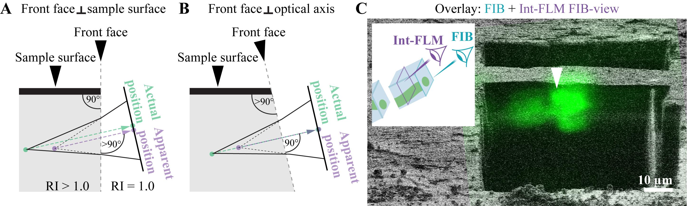
Figure 6. Axial targeting by FIB-view imaging with the int-FLM. (A) If the trenches are milled at a stage tilt of 7° and a stage rotation of 180°, the exposed front face is perpendicular to the sample surface but not normal to the optical axis of the int-FLM. This would distort the axial position of a feature due to refractive index mismatch with a tilted surface. (B) If trench milling is performed so that the front face in lamella milling orientation is perpendicular to the optical axis of the int-FLM, axial targeting can be performed reliably (Capitanio et al.). (C) Overlay of a FIB (gray) and int-FLM FIB-view image recording the cellular autofluorescence (green). Both images were acquired in lamella milling orientation. The junction between cells is marked by a white arrowhead. The inset illustrates the location of the sample surface with respect to the imaging direction of FIB and int-FLM in lamella milling orientation.
F. Waffle milling
1. Apply a thick layer of metal-organic platinum by opening the gas injection system (GIS) 3 × 20 s and 15 s in lamella milling and trench milling orientation, respectively, at the GIS working distance in z.
Note: The GIS working distance and the thickness of the deposited layer of metal-organic platinum may vary between different FIB/SEM microscopes, but they can be estimated as described in General Note 6.
Pause point: After trench milling and GIS coating, grids can be unloaded and stored in grid boxes at liquid nitrogen temperature until further use.
Critical: Unloading and reloading usually change the grid orientation slightly, which may render certain regions of the target area inaccessible and may require additional milling steps. Hence, we prefer to finish waffle milling before unloading.
2. Move the stage into lamella milling orientation at a 20° stage tilt.
Critical: If you did FIB-view imaging, this should be the angle you used for FIB-view imaging. Otherwise, the axial targeting is not reliable.
3. Find the coincidence point on the block containing the target area between the trenches.
4. Remove all material below your target area by FIB milling at 3 nA.
a. Take a FIB image at 3 nA. Can you see the edge at the bottom of the sample (Figure 7A)?
b. If yes, create a cross-section with an xz-dimension of 30 × 2 μm covering all material below the target area, but, if possible, leaving 12 μm to the surface of the sample.
c. If not (Figure 7B), tilt the stage higher until you can see the bottom edge (Figure 7C). Remove the material with a cross-section. Tilt the stage back to 20° and check if you can see the bottom edge now. If yes, continue with F3b. If not, repeat F3c.
Note: If you cannot see the bottom edge at the highest accessible tilt, rotate the stage into trench milling orientation and further elongate the trench on top. In any case, it is safer to make long enough trenches so that the lower edge is visible at shallow angles.
Critical: It is important to remove all material below your lamella. Remaining material in the “shadow” of the actual lamella will likely render cryo-ET data acquisition impossible.
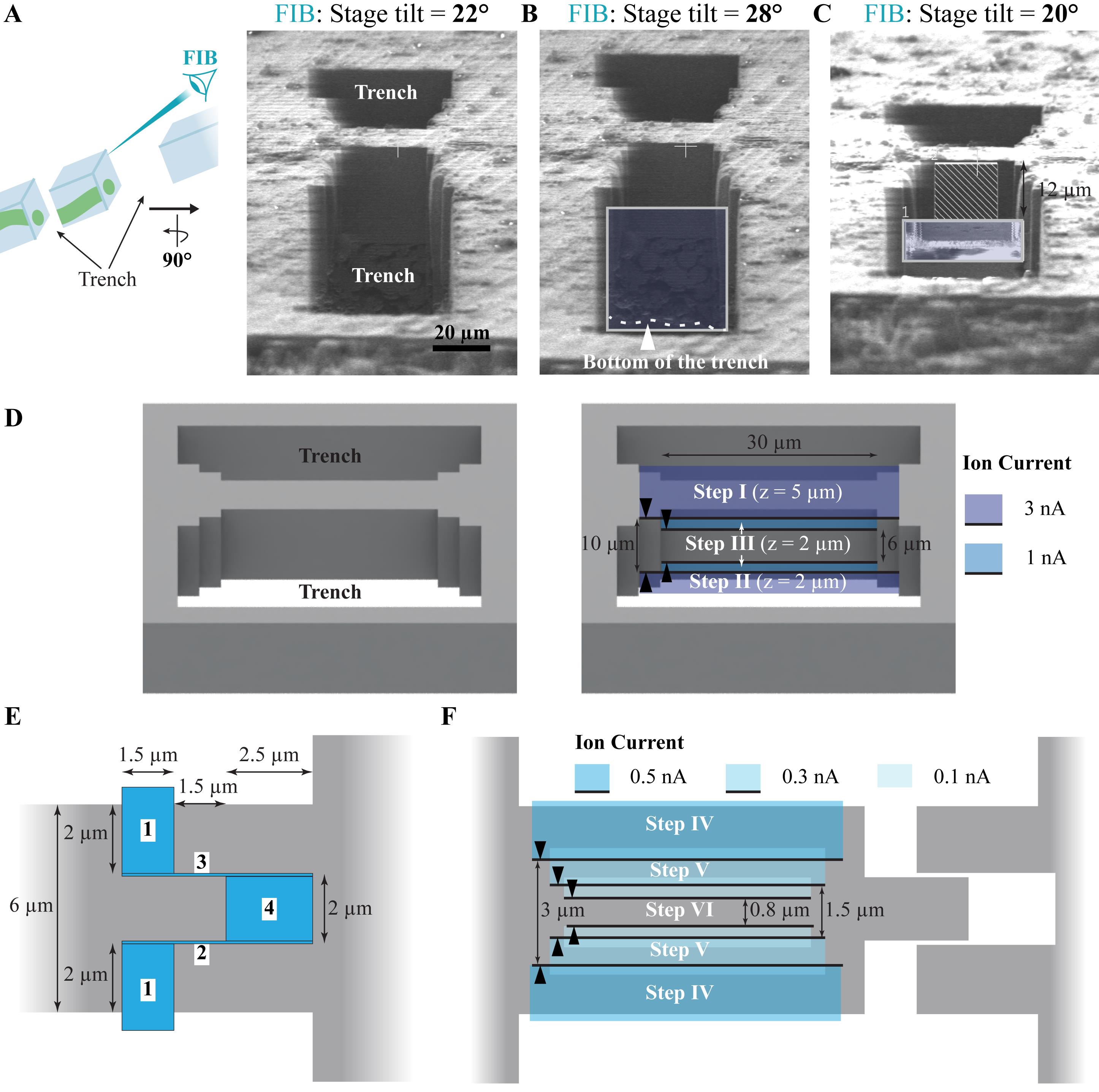
Figure 7. On-grid “waffle” milling. (A–C) Removal of all material below the target area. (A) At a stage tilt of 22°, the bottom of the trench cannot be discerned. The scheme indicates the location of the trenches with respect to FIB imaging direction. (B) At a stage tilt of 28°, the bottom edge of the trench becomes visible (white dashed line). (C) All material below the target area is removed until the bottom of the trench is visible at a stage tilt of 20°, leaving a distance of 12 μm to the sample surface (white rectangle). In (B) and (C), milling patterns are indicated as rectangles with blue shading. (D) Scheme of the prepared lamella site in lamella milling orientation without and with the initial milling patterns in the left and right panels, respectively. (E) Milling patterns for a broad notch. The numbers indicate the milling order of the rectangle patterns. (F) Milling patterns for thinning the lamella after the preparation of the notch. The patterns in (B–D) and (F) are regular cross-sections with the milling direction toward the target area indicated by black arrowheads. The FIB milling patterns are provided in the Supplementary Information.
5. Remove the top surface of the block containing the target area, which is mainly composed of metal-organic platinum at I = 3 nA using a regular cross-section (z = 5 μm; step I in Figure 7D).
6. Thin the lamella to 30 × 10 μm and 30 × 6 μm around the target area at 3 and 1 nA, respectively (z = 2 μm; steps II and III in Figure 7D).
7. Mill a notch similar to the waffle method [13] at a current of 0.5 nA using rectangle patterns (Figure 7E).
a. Record an SEM block face image of the top of the lamella or a top view image with the int-FLM to decide if you want to mill the notch on the left or the right side. It will occupy 6–8 μm of the 30-μm-wide lamella.
b. Mill the two rectangles closest to the target area in parallel (pattern 1 in Figure 7E).
c. Mill the lower vertical pattern (pattern 2 in Figure 7E) followed by the upper one (pattern 3 in Figure 7E).
d. Finish the notch by milling the rectangle furthest away from the target area (pattern 4 in Figure 7E).
Note: For us, a notch allowing for lamella movements of up to 1.5 μm is necessary to prevent lamella bending during fine milling.
8. Successively thin the lamella at 0.5 nA to 3 μm (step IV in Figure 7F), at 0.3 nA to 1.5 μm (step V in Figure 7F), and at 0.1 nA to 0.8 μm thickness (step VI in Figure 7F) using cross sections with xz dimensions of 18–22 × 2 μm.
9. Thin the lamella to a thickness of 250 nm at 50 pA using rectangle patterns milling the top and bottom in parallel (Figure 8A).

Figure 8. Fine milling of waffle lamellae. (A) Thinning of the lamella with two rectangular patterns with a vertical distance of 250 nm milled in parallel. The scheme illustrates the location of the lamella with respect to the FIB imaging direction. (B) Polishing of the lamella from the bottom at a stage tilt of 19°. (C) Polishing of the lamella from the top at a stage tilt of 20.5°. Milling patterns are indicated by blue rectangles; milling directions are indicated by blue arrowheads. The FIB milling patterns are provided in the Supplementary Information.
10. Switch to an ion current of 30 pA. Tilt the stage to 19° and 20.5–21° and polish the lamella only from the bottom (Figure 8B) and the top (Figure 8C), respectively.
Notes:
1. Cross-section patterns deplete material faster and generate smoother surfaces. But they typically provide a substantially slower readout than rectangle patterns. The fast readout is crucial when you thin the lamella to its final thickness. Sometimes, the lamella deforms or starts tearing. When this happens, milling must be stopped or interrupted to re-adjust patterns. Thus, we prefer to use cross-sections for initial “rough” milling steps and use rectangular patterns only for the final thinning and polishing steps.
2. Recording low-current FIB and SEM images regularly helps to understand if your lamella starts breaking. Recording a movie of FIB images (saving frames every 2–5 s) during the last milling steps can be helpful for troubleshooting if something goes wrong.
11. (Optional) Sputter a thin layer of metallic platinum on the sample to increase conductivity and suppress charging-related artifacts (movement, warping) during TEM tilt-series acquisition (e.g., U = 1 kV, I = 10 mA, p = 0.2 mbar, t = 2–4 s).
Note: On our systems, this condition also deposits platinum particles with diameters of 5–15 nm on the lamella surface. They can serve as fiducials for tilt-series alignment, generating higher-quality tomograms than patch tracking–based approaches, specifically in regions devoid of high-contrast cellular features.
12. Unload the sample and store it until transfer into a transmission electron microscope.
Part II. Serial lift-out with double-sided attachment from below
Note: The redeposition milling technique used here to attach different materials works best if the surfaces of the attachment sites are smooth. This is achieved by polishing the respective surfaces with cross-sections.
A. Prepare for the lift-out session at room temperature
1. Load a 400 × 100 mesh grid into the FIB/SEM instrument.
a. Clip the grid into a TEM cartridge without a cutout for FIB milling. The shiny top of the grid must face down during clipping so that it is the top when loaded into the FIB/SEM instrument.
Critical: If the grid was bent during clipping, discard it. A bent grid may render the attachment later in the workflow difficult or even impossible.
b. Label the top of the cartridge on both sides along the 100 mesh bars with two blue marks and the opposing sides along the 400 mesh bars with a black and a red mark (Figure 9A).
Critical: Use a magnifying glass or a stereomicroscope to add the marks precisely along the directions of the grid bars. The marks will help you to align the grid when loading into the FIB/SEM instrument. Proper grid alignment is crucial for the success of lift-out with double-sided attachment.
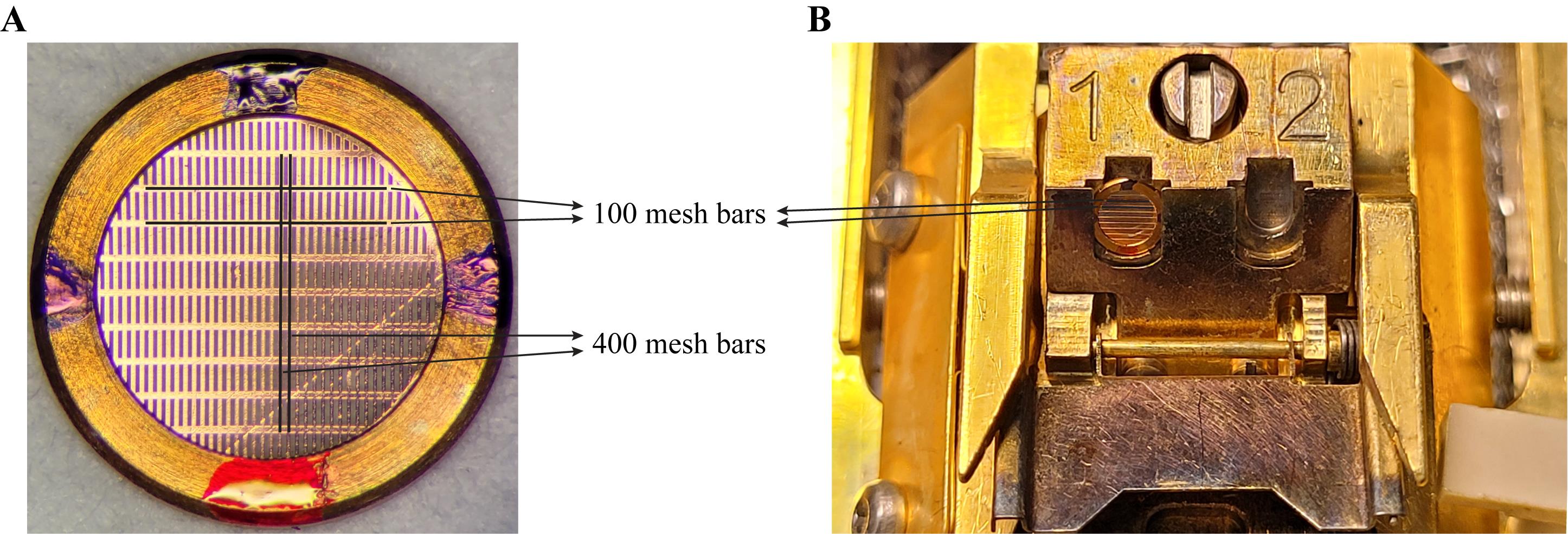
Figure 9. Labeling and mounting 400 × 100 mesh grids. (A) Labeled cartridge of a clipped 400 × 100 mesh grid with two blue marks on either side along the 100 mesh bars, as well as a black and a red mark on opposite sides along the 400 mesh bars. (B) Mounted grid into the FIB shuttle with the 100 mesh bars aligned horizontally and the red mark facing down.
c. Mount the clipped 400 × 100 mesh grid into the FIB shuttle. The 100 mesh bars indicated by the blue markers must be aligned horizontally, and the red marker should face down. Load the shuttle into the FIB/SEM instrument at room temperature (Figure 9B).
2. Polish the bottom edge of the EasyLift needle.
a. Insert the needle into the parking position and move it into the coincidence point of FIB and SEM.
b. Coarsely remove the remainders of previous lift-out experiments at 5–30 nA (Figure 10).
Note: If a copper adapter with a height of at least 10 μm is attached to the needle, it can be reused as described below.
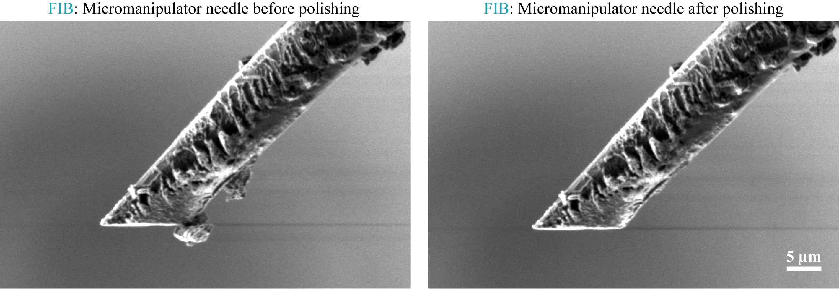
Figure 10. Polish the bottom of the needle. The needle before and after polishing its bottom in the left and right panels, respectively.
c. Polish the bottom of the needle at 1 nA with a cross-section across the full width of the needle, with the milling direction toward the needle. Set the z-dimension of the cross-section to roughly the diameter of the needle at the tip.
d. Retract the needle.
3. Prepare and attach a copper adapter for the needle following the scheme in Figure 11A.
a. Move the stage into trench milling orientation (stage tilt = 7°, relative rotation = 180°).
b. Find the coincidence point of FIB and SEM on a 100 mesh bar between two 400 mesh bars (inset in Figure 11B).
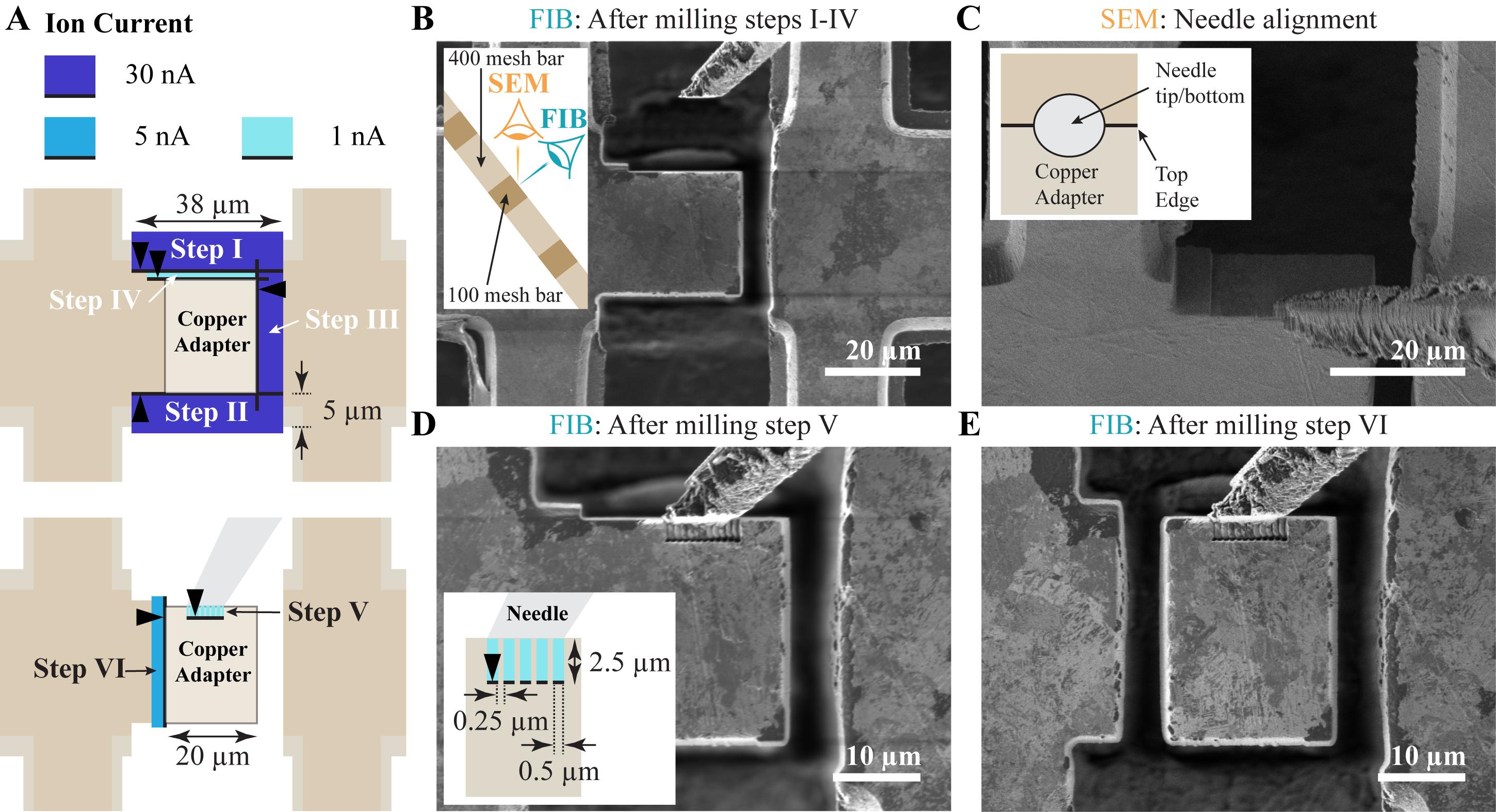
Figure 11. Preparation of a copper adapter from a 400 × 100 mesh grid. (A) Scheme of the milling patterns. All milling patterns are cross-sections with the black arrowheads indicating the milling direction. (B) FIB image after milling steps I–IV. The inset illustrates the location of 400 and 100 mesh bars with respect to the FIB and SEM imaging directions. (C) SEM image of the needle bottom centered on the top edge of the copper adapter. The inset depicts how the bottom of the needle was positioned with respect to the copper adapters’ top edge. (D) FIB image of the needle attached to the copper adapter by redeposition milling. The inset shows the dimensions of the cross-section patterns used for redeposition milling. The “multi pass” parameter is set to 1. The milling direction is indicated by a black arrowhead. An array of 15–25 of these cross-sections is placed along the interface between the needle’s bottom edge and the copper adapter. (E) FIB image of the detached copper adapter. The FIB milling patterns are provided in the Supplementary Information.
c. Remove 4 μm from the top and bottom of the grid bar using cross-sections with xyz-dimensions of 38 × 5 × 20 μm and a milling direction toward the center of the grid bar at 30 nA.
d. Detach the copper adapter on one side with a 5 × 35 × 70 μm cross-section, milling toward the adapter.
e. Polish the top of the copper adapter at 1 nA (cross section, xyz size = 25 × 1.5 × 20 μm; Figure 11B).
f. Insert the polished needle.
g. In the SEM, adjust the position of the needle only in x and y so that the center of its tip aligns with the top edge of the copper adapter (Figure 11C). The polished needle face needs to form a step with the copper adapter to allow for effective redeposition and attachment.
h. In the FIB, bring the needle in contact with the upper surface of the copper adapter, moving only in z.
i. Define a horizontal array of 15–25 cross-sections with xyz-dimensions of 0.5 × 2.5 × 4 μm every 250 nm and place it along the interface between needle and adapter on the adapter with the milling direction away from the needle.
Critical: Set the “multi pass” parameter for cross-sections used for redeposition milling to 1!.
Critical: Adjust the spacing of the patterns depending on the alignment quality of the ion beam. Space the patterns further apart if single attachment patterns overlap too much, forming a continuous attachment groove.
j. Mill the pattern array at 1 nA to attach the needle to the copper adapter (Figure 11D).
Note: Move the needle one 500 nm step upward in z. You should see no movement, or a movement of the entire grid. If only the needle moves, the attachment was not successful.
k. Detach the copper adapter with a 5 × 35 × 70 μm cross-section at 5–30 nA, resulting in a final adapter width of 15–20 μm (Figure 11E). Ensure that detachment was successful by moving a 500 nm step in z. Now, only the adapter should move.
l. Polish the lower edge of the copper adapter at 1 nA (cross section, xyz-dimensions: 16–21 × 1.5 × 20 μm).
Note: Polishing the bottom of the copper adapter can also be performed after the system has been cooled down, right before the lift-out experiment starts.
m. Retract the needle.
4. (Optional) Prepare the copper adapter for reuse (Figure 12).
Note: Copper adapters can be used for several lift-out experiments.
a. Coarsely remove the old attachment site at 5–30 nA.
b. Polish the lower edge of the adapter at 1 nA (cross section, xyz-dimensions: 16–20 × 1.5 × 20 μm).
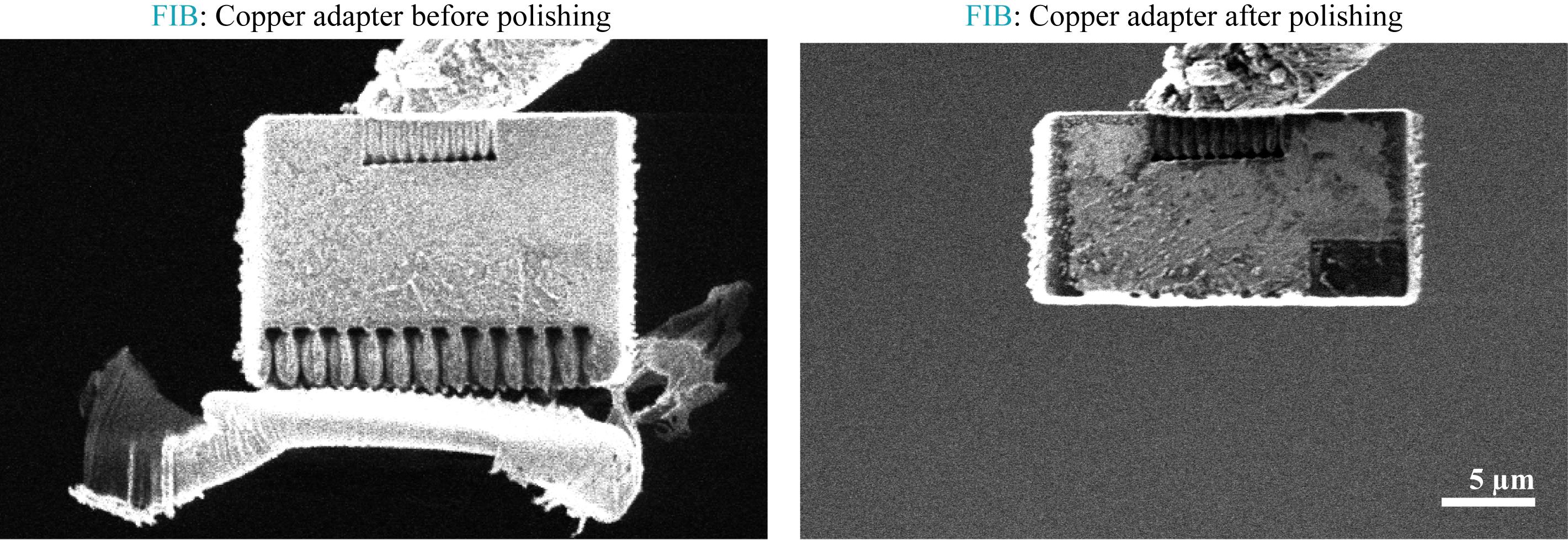
Figure 12. Reuse of the copper adapter. The copper adapter with remnants of a previous lift-out experiment before and after polishing for reuse, shown in the left and right panels, respectively.
5. Mill cavities for the attachment from below into the receiver grid (Figure 13).
a. If necessary, precisely align the 400 mesh bars vertically by rotating the stage.
b. With the stage in trench milling orientation, find the coincidence point of FIB and SEM in the center of the grid.
Critical: Only regions within about 1 μm from the grid center are accessible with the stage movement of a Titan Krios. Hence, cavities and attachment sites must be within that range.
c. Mill rectangular 8 × 90 μm cavities into neighboring 400 mesh bars at 30 nA using cross-sections with xyz-dimensions of 9 × 90 × 25 μm. The milling direction is parallel to the bar from the mesh hole toward the bar. The lower edge of the patterns should be in the middle of the grid rectangles (Figure 13).
d. Unload the grid and store it until it is used for a lift-out experiment.
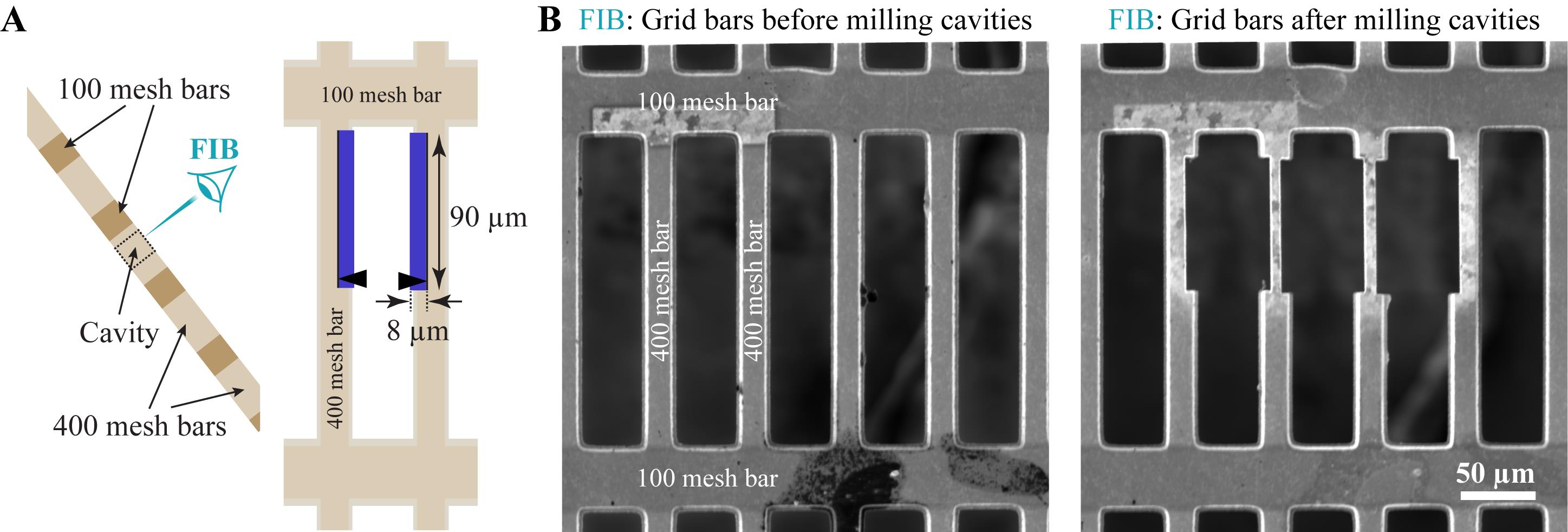
Figure 13. Preparation of cavities for attachment from below. (A) Scheme illustrating the preparation of the cavities. The left scheme shows the location of cavities with respect to grid bars and the FIB imaging direction. The right scheme depicts the dimensions of the milling patterns as blue rectangles with the milling direction indicated by black arrowheads. (B) Grid bars before and after milling the cavities in the left and right panels, respectively.
B. Perform the lift-out
1. Load the modified 400 × 100 mesh receiver grid and the sample for lift-out into the FIB/SEM instrument.
a. Mount the modified receiver grid into the FIB shuttle with the loading station at room temperature. Make sure the 100 mesh bars indicated by the blue marks are precisely aligned horizontally. Fix the grid in the shuttle by closing the shuttle clamp.
b. Cool down the loading station.
c. Open the shuttle clamp and load the sample for lift-out into the free slot of the shuttle. Then, close the clamp again.
d. Load the shuttle into the cooled FIB/SEM instrument.
Note: Orienting the receiver grid is much easier at room temperature than in the cold state.
Critical: The 100-mesh bars must be aligned horizontally. For an alignment error below 10°, stage rotation may be used to compensate for remnant misalignment. For alignment errors above 10°, the receiver grid needs to be unloaded and its rotation manually re-adjusted to avoid large tomogram x-tilts (perpendicular to the tilt axis of the tilt-series).
2. Perform targeted trench milling as described in section D. The final width (x-dimension) of the target area, however, must be larger than for the previously described workflow (i.e., 60–65 μm).
Critical: Extending the width of the target volume is vital for double-sided attachment. After detachment from the bulk sample, it must still be wide enough to span the mesh between the two attachment sites. For double-sided attachment from below, this gap is about 55 μm wide. Another 5–10 μm is needed for the attachment. It is better to lift out a slightly too wide block, as its width can always be reduced. Once the lift-out block becomes too narrow, the experiment fails.
3. Lift-out option I: With the stage in trench milling orientation similar to [1], resulting in sectioning transverse to the sample surface (Figure 14A).
a. Insert the EasyLift needle after trench milling with the stage still in trench milling orientation.
b. If not yet done, polish the lower edge of the copper adapter at 1 nA with a cross-section (z-dimension = 10 μm).
c. In the SEM, position the bottom face of the copper adapter in the center of the block face.
d. In the FIB, bring the copper adapter in contact with the top block face.
e. Define a horizontal array of cross-sections with xyz-dimensions of 0.5 × 2.5 × 4 μm every 250 nm and place it along the interface between the copper adapter on the block containing the target area on the adapter with the milling direction away from the block (Figure 14B).
Critical: Set “multi pass” to 1 for the cross-sections used for redeposition milling.
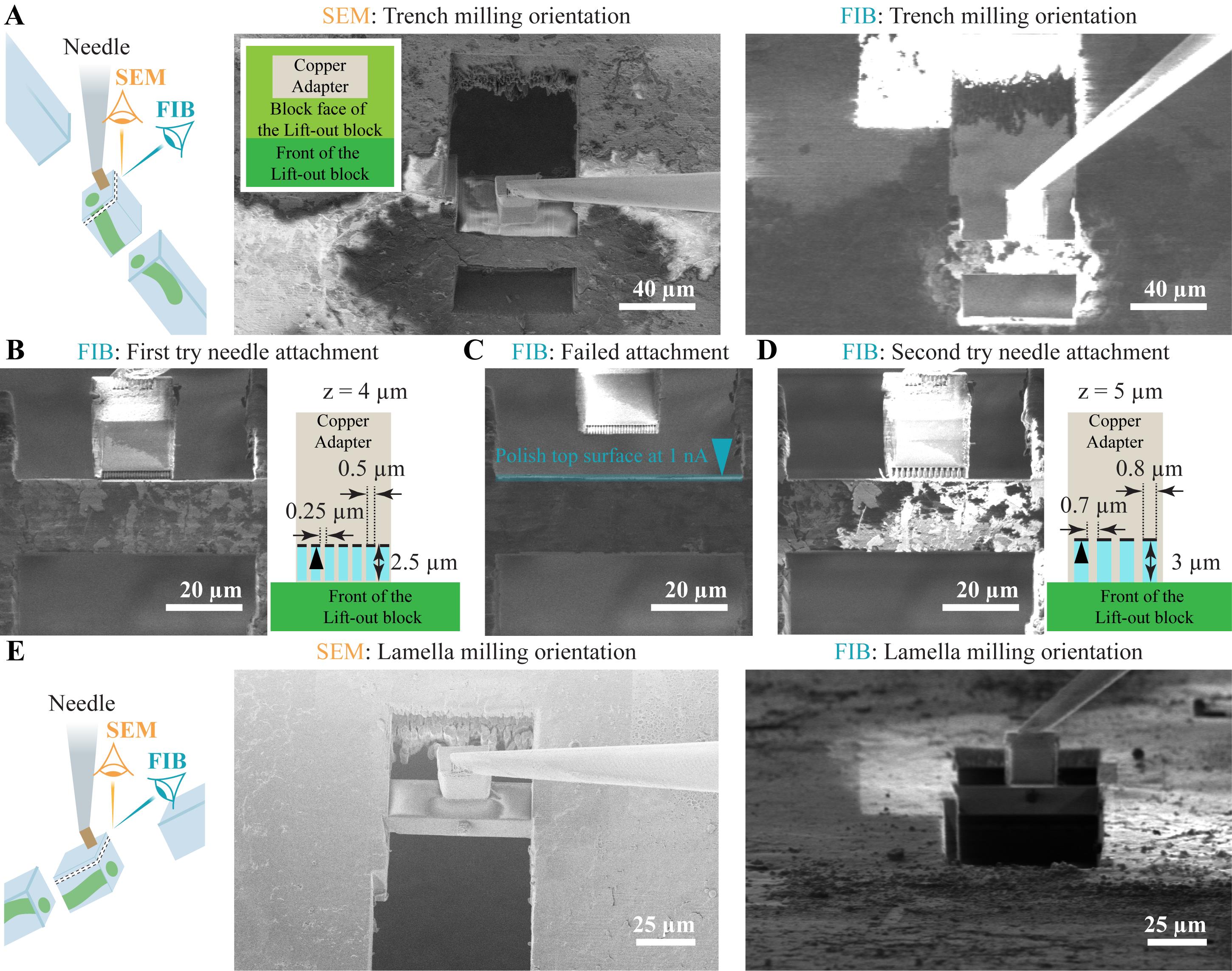
Figure 14. Lift-out in different stage orientations. The schemes on the left illustrate the orientation of sections marked by black, dashed lines with respect to the imaging directions of FIB and SEM. (A) Lift-out in trench milling orientation. The middle panel shows an SEM image with the needle attached to the lift-out block. The inset illustrates the positioning of the copper adapter with respect to the milled front of the block. The right panel shows an FIB image. (B) FIB image of the copper adapter attached to the lift-out block. The inset illustrates the dimensions of the cross-sections (“multi pass” set to 1) used for the attachment. The milling direction is indicated by a black arrowhead. (C) If the attachment fails, retract the needle and polish the top surface of the lift-out block. The milling pattern is indicated by a blue rectangle and the milling direction by a blue arrowhead. (D) FIB image after the second attempt to attach the copper adapter. The inset shows the dimensions of the cross-sections (“multi pass” set to 1) used for the second attachment. The milling direction is indicated by a black arrowhead. (E) Lift-out in lamella milling orientation. SEM and FIB images are shown in the middle and right panels, respectively. The copper adapter is positioned in the center of the top of the lift-out block. The FIB milling patterns are provided in the Supplementary Information.
f. Mill the pattern array at 1 nA to attach the lift-out block to the copper adapter.
Note: Move the needle 500 nm upward. You should see no movement or a movement of the entire grid. If only the needle moves, the attachment was not successful.
g. If the attachment was not successful, retract the needle 10–20 μm.
h. Polish the top surface of the lift-out block and the bottom of the copper adapter at 1 nA with cross-sections (z = 5 μm, Figure 14C).
i. Define a horizontal array of cross-sections with xyz-dimensions of 0.8 × 3 × 5 μm every 700 nm and place it along the interface between the copper adapter on the block containing the target area on the adapter with the milling direction away from the lift-out block (Figure 14D).
Critical: Set “multi pass” to 1 for the cross-sections used for redeposition milling.
j. Mill the pattern array at 1 nA to attach the block to the copper adapter.
Note: Move the needle 500 nm upward. You should see no movement or a movement of the entire grid. If only the needle moves, the attachment was not successful.
k. Detach the lift-out block on both sides by milling cross-sections (xz-dimension = 5 × 5 μm) at 5 nA with the milling direction toward the lift-out block.
Critical: The distance between the two patterns determines the width of the lift-out block. For the double-sided attachment from below, it must be around 55 μm.
Note: Move the needle 500 nm upward. You should see a movement of the needle and the lift-out block. If only the needle moves, the attachment to the block did not hold. If nothing or the whole grid moves, the lift-out block is still attached to the bulk sample.
l. Move the needle up in z and pay attention to not crash the lift-out block into the top edge of the trench.
Note: The movement of the needle out of the sample is neither a pure y nor a pure x movement. Small iterative movements in both directions need to be performed to move the lift-out block out of the sample bulk. As a consequence, the movements must be controlled regularly by FIB and SEM imaging. Start with upward movements in z (500 nm to 1 μm steps). After the volume has noticeably separated from the bulk, it may be moved forward in y.
m. Retract the needle to bring the lift-out block into a safe position and allow for stage movement.
4. Lift-out option II: In lamella milling orientation, resulting in sectioning nearly parallel to the sample surface (Figure 14E).
a. After trench milling, move the stage into the lamella milling orientation and find the coincidence point of FIB and SEM on the block containing the target area.
Note: Locate your target area in z, if not yet done so, by SEM block face imaging or FIB-view imaging as described in section E.
Critical: The bottom edge of the block must be discernible in FIB images in this orientation. If not, tilt the stage to a higher angle or extend the top (front) trench in trench milling orientation.
b. Apply a thick layer of metal-organic platinum by moving the stage in lamella milling orientation to the GIS working distance and opening the GIS for 3 × 30 s.
Critical: This process will protect the front of the lift-out block that was exposed through trench milling. This layer will be continuously imaged during lift-out and subsequent sectioning. If it is too thin, the lamella front will be damaged, resulting in problems during lamella preparation (see also Troubleshooting point 5).
c. Remove the uppermost layer, including the rough grid surface at 3 nA using a cross-section (z-dimension = 5 μm).
d. Coarsely remove all material above and below the target area at 3 nA (cross-sections, z-dimension = 2 μm) as determined by the target area axial localization.
e. Polish the top edge of the block at 1 nA (cross-sections, z-dimension = 3 μm, milling direction toward the target area).
Critical: This surface must be smooth. It will be attached to the copper adapter, and redeposition milling is more successful if the attached surfaces are smooth.
f. Insert the EasyLift needle with the stage in lamella milling orientation.
g. If not yet done, polish the lower edge of the copper adapter at 1 nA with a cross-section (z-dimension = 10 μm).
h. In the SEM, position the bottom front of the copper adapter in the center of the lift-out block.
i. In the FIB, bring the copper adapter in contact with the lift-out block.
j. Define a horizontal array of cross-sections with xyz-dimensions of 0.5 × 2.5 × 4 μm every 250 nm and place it along the interface between the copper adapter on the block containing the target area on the adapter with the milling direction away from the block (Figure 14B).
Critical: Set “multi pass” to 1 for the cross-sections used for redeposition milling.
k. Mill the pattern array at 1 nA to attach the block to the copper adapter.
Note: Move the needle 500 nm upward. You should see no movement or a movement of the entire grid. If only the needle moves, the attachment was not successful.
l. (Optional) If the attachment was not successful, retract the needle in z by 10 μm. Polish the top of the lift-out block at 1 nA. Bring the copper adapter into contact with the lift-out block. Define a horizontal array of cross-sections with xyz-dimensions of 0.8 × 3 × 5 μm every 700 nm. Place it along the interface between the copper adapter and the lift-out block on the copper adapter (Figure 14D). Mill at 1 nA.
m. Detach the lift-out block on both sides by milling cross-sections (xz-dimension = 5 × 5 μm) at 5 nA with the milling direction toward the lift-out block.
Critical: The distance between the two patterns determines the width of the lift-out block. For the double-sided attachment from below, it must be around 55 μm.
Note: Move the needle 500 nm upward. You should see movement of the needle and the lift-out block. If only the needle moves, the attachment to the block did not hold. If nothing or the whole grid moves, the lift-out block is still attached to the bulk sample.
n. Retract the needle.
C. Lift-in
1. Move the stage in lamella milling orientation (stage tilt = 15°) to the modified 400 × 100 mesh grid.
2. Precisely align the 100-mesh bars horizontally using the stage tilt. If the initial alignment error is larger than 10°, unload the receiver grid and adjust its orientation manually.
3. Find the coincidence point of FIB and SEM in the back of the cavities between the two grid bars.
4. Prepare the plateaus for the attachment from below.
a. FIB mill cross-sections with xyz-dimensions of 9 × 10 × 20 μm on both bars at the back of the cavity at 30 nA (milling direction top to bottom). The bottom edges of the cross-sections must be aligned to the same height. The top edge of the patterns must be at least 1 μm above the edge of the grid surface and cavity (Figure 15A).
b. Smooth the top edge of the plateaus with two normal patterns milled in parallel on either side (I = 15 nA, xyz-dimensions = 9 × 1 × 20 μm, milling direction top to bottom; Figure 15B).
Critical: The patterns must be milled in parallel. This ensures that the plateaus have the same height on both sides, even if the stage is drifting during plateau preparation (Figure 15C).
Note: The width of the resulting attachment site on 400 × 100 mesh grids is between 50 and 55 μm. The block containing the target area that is lifted out must overlap with the plateaus on both sides at least 3 μm for the attachment from below.
c. Repeat this for all cavities.
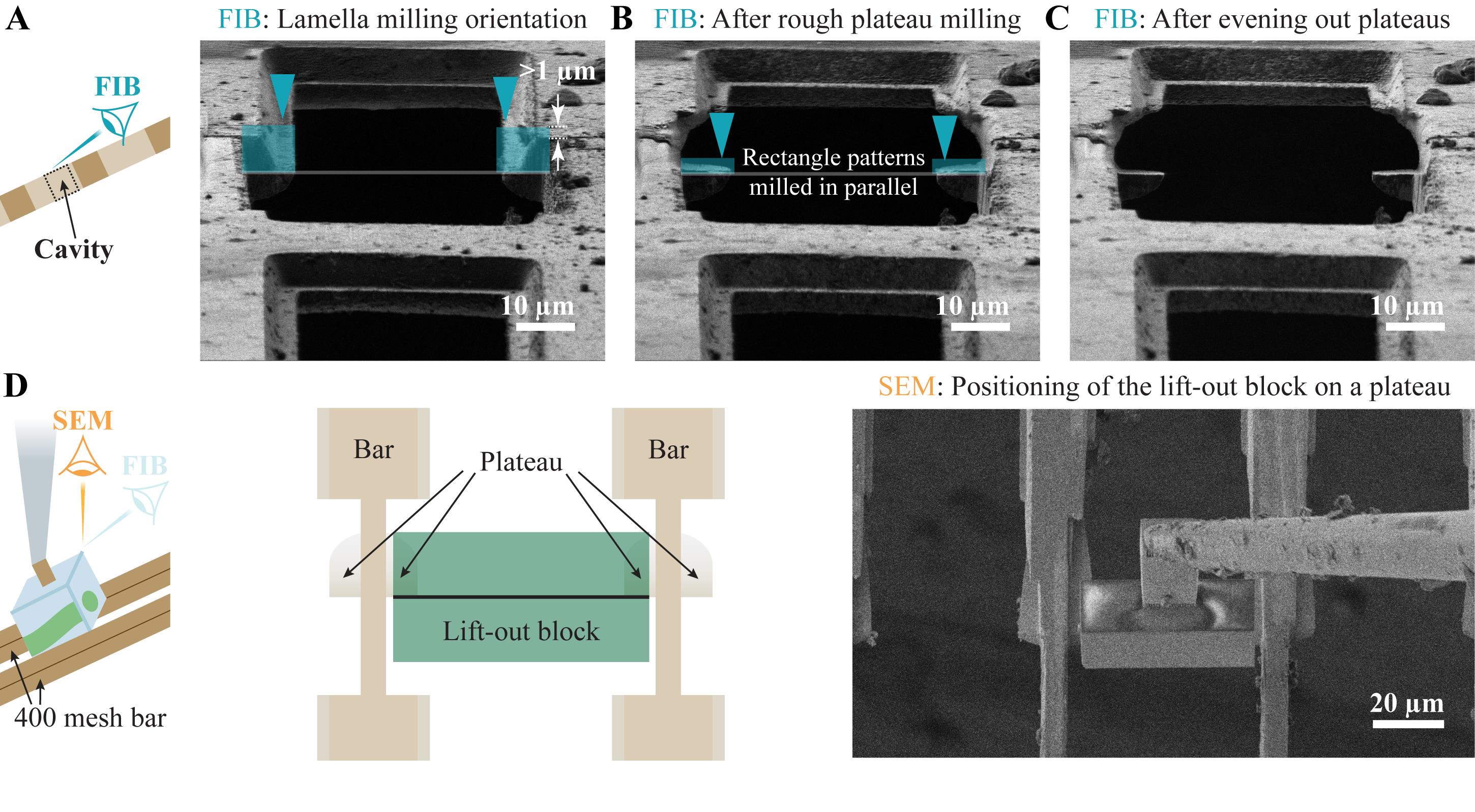
Figure 15. Preparation of plateaus for the attachment from below. (A) Coarse milling of the plateaus. The scheme illustrates the location of the cavity with the stage in lamella milling orientation with respect to the FIB imaging direction. (B) FIB image after coarse milling of plateaus. To even out height differences between plateaus, two rectangular patterns are milled in parallel. In (A) and (B), milling patterns are indicated by blue rectangles and the milling direction by blue arrowheads. The grey line emphasizes that the lower edges of milling patterns must be aligned. (C) FIB image after completion of the plateau preparation. (D) Alignment of the lift-out block for the attachment from below relative to the plateaus. The scheme on the left depicts the location of the lift-out block with respect to the SEM imaging direction. The scheme in the middle and the SEM image in the right show how the lift-out block is aligned with respect to the plateaus. The FIB milling patterns are provided in the Supplementary Information.
5. Insert the needle with the lift-out block attached to it.
6. In the SEM, align the center of the lift-out block to the front edge of the plateaus (Figure 15D).
7. Trim the lift-out block to fit on the plateaus.
a. In the FIB, move the needle down until the lift-out block is 10 μm above the plateaus.
b. If the lift-out block is wider than the plateaus, trim it on both sides (Figure 16A) with cross-sections at 1 nA (z-dimension = 2 μm, milling direction toward the lift-out block).
Critical: The lift-out block should overlap with the plateaus at least 3 μm on either side. This ensures stable attachment.
Critical: The gap between the lift-out block and the grid bars next to the plateaus should be larger than 500 nm on either side, which prevents problems during sectioning.
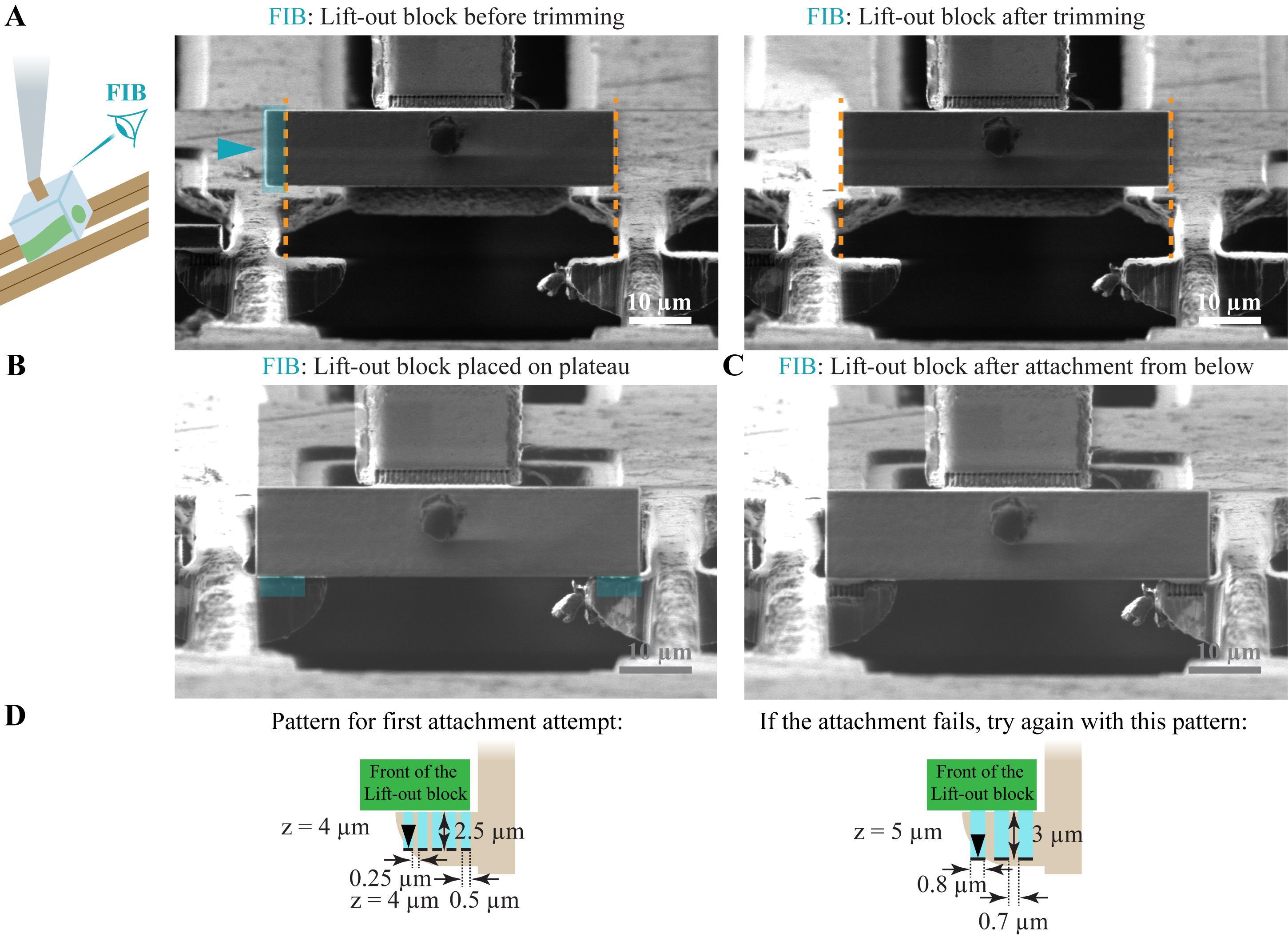
Figure 16. Attachment of serial lift-out sections from below. (A) The lift-out block before and after trimming to fit on the plateaus in the left and right panels, respectively. A milling pattern is indicated by a blue rectangle, its milling direction by a blue arrowhead, and lines used for lift-out block alignment as orange, dashed lines. The scheme on the left illustrates the location of the lift-out block with respect to the FIB imaging direction. (B) The lift-out block, placed on the two plateaus. Attachment sites are marked with blue rectangles. (C) FIB image after attachment from below. (D) Scheme of the cross-section arrays (“multi pass” set to 1) used for attachment for the first and second attempts in the left and right panels, respectively. The milling directions are indicated by black arrowheads. The FIB milling patterns are provided in the Supplementary Information.
c. Smooth the lower edge of the lift-out block at 1 nA (z-dimension = 2 μm, milling direction toward the needle).
8. Generate the serial sections.
a. Place the lift-out block on the plateaus by moving down the needle while imaging in the FIB.
b. Define two horizontal arrays of six cross-sections with xyz-dimensions of 0.5 × 2.5 × 4 μm every 250 nm and place them along the interfaces between the two plateaus and the lift-out block on the plateaus with the milling direction away from the block (Figure 16B).
Critical: Set “multi pass” to 1 for the cross-sections used for redeposition milling.
c. Mill the pattern array at 1 nA to attach the lift-out block from below (Figure 16C, D).
Note: Move the needle 500 nm upward. You should see no movement or a movement of the entire grid. If only the lift-out block moves, the attachment was not successful.
d. (Optional) If the attachment was not successful, define two horizontal arrays of three cross-sections with xyz-dimensions of 3 × 0.8 × 5 μm every 700 nm. Place them along the interfaces between the two plateaus and the lift-out block on the plateaus with the milling direction away from the block. Set the milling direction away from the block (Figure 16D). Mill at 1 nA.
e. Define a horizontal line pattern (z-dimension = 10 μm) that is 2 μm wider than the lift-out block and place it 3 μm higher than the lower edge of the lift-out block (Figure 17).
Note: The positioning of the line pattern above the lower edge of the lift-out block defines the section thickness. Thicker sections reduce the contextual information. Thinner sections are possible (1.5–2 μm), but that complicates the subsequent section trimming step.
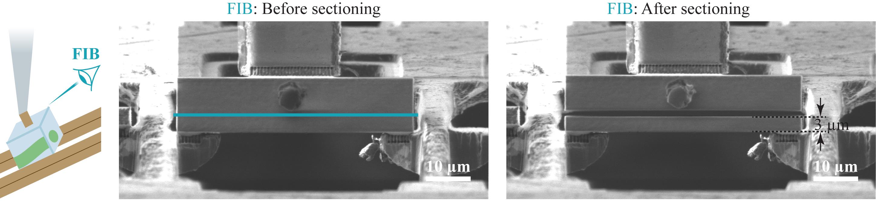
Figure 17. Sectioning of the lift-out block. The left panel illustrates the location of the lift-out block with respect to the FIB imaging direction. The lift-out block before and after sectioning is shown in the middle and right panels, respectively. The line pattern used for sectioning is indicated as a blue line and the section thickness by black dashed lines. The FIB milling patterns are provided in the Supplementary Information.
f. Mill the line pattern at 1 nA.
Note: Afterward, move the needle 500 nm upward. You should see movement of the needle and the remaining lift-out block. If nothing or the whole grid moves, the lift-out block is still attached to the section.
g. Retract the needle and move to the next attachment site.
9. Repeat step C8 until the whole lift-out block is sliced up.
D. Trim the sections
1. Record top-view images with the int-FLM of all sections with the stage in trench milling orientation.
a. Use the reflected light channel to focus on the section
b. Record a z-stack with reflected light and cellular autofluorescence channel as for targeted trench milling (bin = 4, 10 z-slices, z-step = 1 μm).
2. Identify sections that do not contain the target area based on the int-FLM top views. These sections can be skipped in the next steps (Figure 18A).
3. For sections that contain the target area, identify the regions of the sections that do not contain the material of interest based on the int-FLM top views.
4. Apply a layer of metal-organic platinum by opening the GIS 15 s in trench milling orientation at the GIS working distance in z.
5. For every section, remove material above and below the target area with the stage in trench milling orientation. Use cross-sections (z-dimension = 1 μm) milled at 3 nA with the milling direction toward the target area.
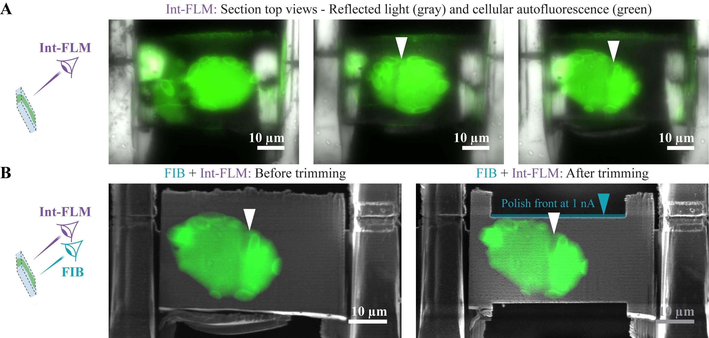
Figure 18. Trimming of serial lift-out sections. The schemes on the left illustrate the orientation of sections with respect to the imaging directions of FIB and int-FLM. (A) Top views recorded with the int-FLM of three successive serial lift-out sections. Shown is the reflected light channel (gray) and cellular autofluorescence (green). The junction between cells is only contained in two of them, as indicated by the white arrowheads. (B) The section in the right panel in (A) before and after trimming in the left and right panels, respectively. Depicted is the overlay of an FIB image (gray) and cellular autofluorescence recorded with the int-FLM (green), both recorded in trench milling orientation. The FIB milling patterns are provided in the Supplementary Information.
6. Polish the top front at 1 nA (cross-sections, z-dimension = 2 μm, Figure 18B).
Critical: During trimming, at least 1–2 μm should be removed from the top edge. This surface was constantly exposed to the FIB during lift-out, lift-in, and sectioning. Thus, it is damaged and uneven.
7. Open the GIS in trench milling and lamella milling orientation for 15 s and 3 × 20 s, respectively, both at the GIS working distance in z.
Note: The trimming minimizes the size of the lamella, which makes fine milling faster and generates smooth section fronts covered with a thick, homogeneous layer of metal-organic platinum, which is key to obtaining homogeneously thin lamellae.
Pause point: Unload the grid after sectioning, section trimming, and GIS coating. Store the receiver grid in a grid box and recover the lift-out sample. Store both at liquid nitrogen temperature.
Critical: If the grid is misoriented upon reloading, sections must be oriented horizontally by rotating the stage. This, in turn, will add an additional x-tilt to tomograms recorded on lamellae, which is not desirable. If the alignment error is larger than 10°, unload the receiver grid, reorient, and reload it.
Critical: Every additional unloading and reloading step bears the risk of losing sections or even destroying them all if mistakes occur while handling grids manually with tweezers.
E. Fine milling for all sections containing the target area
1. Remove the top and bottom of the section over its whole width at 1 nA using cross-sections (top z-dimension = 5–6 μm, bottom z-dimension = 2 μm, vertical distance between patterns = 2 μm; Figure 19A).
Note: The top layer of the section is composed of metal-organic platinum and requires longer milling times.
2. (Optional) Record an SEM block-face image of the section surface. It can reveal the location of the target area (Figure 19B).
3. Adjust the width and position of the milling patterns to be centered around the target area.
Critical: Keep the width of the lamella for fine milling as small as possible. This speeds up the milling process and increases the success rate.
4. Thin the lamella to 1.5 μm and 0.8 μm at ion currents of 0.3 and 0.1 nA, respectively, using cross-sections (similar to Figure 7F; z-dimension = 2 μm, milling direction toward the center of the lamella).
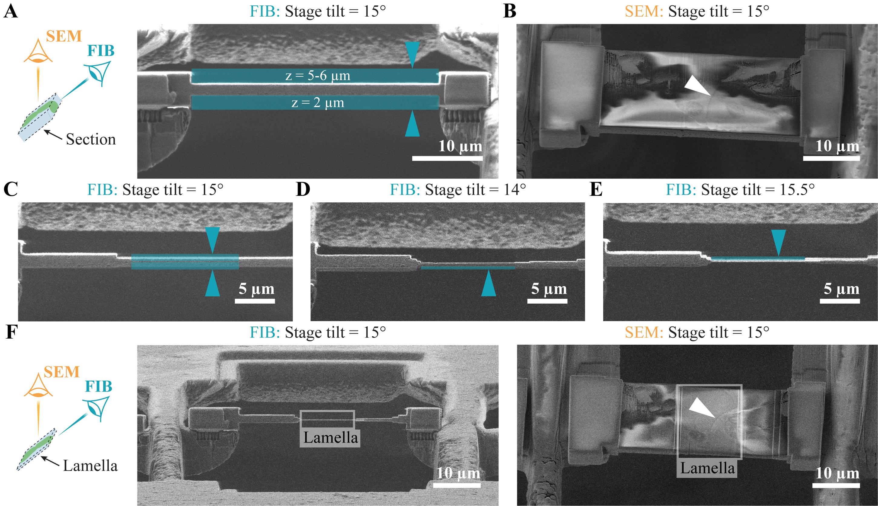
Figure 19. FIB milling of serial lift-out sections. The schemes on the left illustrate the location of the section or lamella with respect to the FIB/SEM imaging direction. (A) The first fine milling step at 1 nA. (B) SEM block face image after removing the thick layer of metal-organic platinum on top of the section in (A). (C) Fine milling of the section with two rectangular patterns with a vertical distance of 200 nm milled in parallel. (D) Polishing of the lamella from the bottom at a stage tilt of 14°. (E) Polishing of the lamella from the top at a stage tilt of 15.5°. (F) FIB and SEM images of the final lamella in the left and right panels, respectively. Milling patterns are indicated by blue rectangles, the milling directions by blue arrowheads, and the junction between cells by white arrowheads. The FIB milling patterns are provided in the Supplementary Information.
5. Thin the lamella to a thickness of 200 nm at 50 pA using rectangular patterns milled in parallel (Figure 19C).
6. Switch to an ion current of 30 pA. Tilt the stage to 14° and 15.5° and polish the lamella only from the bottom (Figure 19D) and the top (Figure 19E), respectively.
Notes:
1. Cross-sections deplete material faster and generate smoother surfaces. But, in contrast to rectangular patterns, they do not provide an immediate readout or image. This immediate readout is crucial when you thin the lamella to its final thickness. Sometimes, the lamella deforms or starts breaking, and you must interrupt milling. Thus, we prefer cross-sections for all initial milling steps and use rectangular patterns only for the final thinning steps.
2. Taking regular FIB and SEM images helps to understand if your lamella starts breaking. Recording a movie in the FIB channel (saving frames every 2–5 s) during the last milling steps can be beneficial for troubleshooting if something goes wrong.
7. (Optional) Sputter a thin layer of metallic platinum on your sample (U = 1 kV, I = 10 mA, p = 0.2 mbar, t = 2–4 s).
Note: On our systems, this introduces spherical platinum particles with diameters of 5–15 nm on the lamella surface. They can be used as fiducials for tilt-series alignment. In our hands, that generates higher-quality tomograms than patch tracking–based approaches.
8. Unload the sample and store it until it is imaged in a transmission electron microscope.
Part III. Serial lift-out with double-sided attachment from the side
Note: The serial lift-out with double-sided attachment from the side was described previously [1]. The attachment from the side has a higher throughput than the attachment from below because the time-consuming plateau preparation is omitted. It requires, however, more precision and user expertise.
A. Prepare the lift-out session at room temperature
1. Clip, label, and load a 400 × 100 mesh grid and attach a copper adapter to the EasyLift needle as described in sections A1–4.
2. Mill marker lines for the alignment of the lift-out block (Figure 20).
a. Move the stage into trench milling orientation.
b. Precisely align the 100-mesh bars horizontally by rotating the stage.
c. Find the coincidence point of FIB and SEM in the center of the lower grid half, three or four 100-mesh bars from the grid’s lower edge.
d. Define cross-sections with yz-dimensions of 2 × 12 μm across the center of 400-mesh bars (milling direction top to bottom) over the whole width of the grid bar.
e. Mill the marker lines at 15 nA.
Note: Milling extended cross-sections takes longer than the line patterns used in the original publication [1], but broader marker lines are easier to see in SEM and FIB, even if the image quality is bad, which makes the experiment easier.
f. Store the modified 400 × 100 mesh receiver grid until it is used for a lift-out experiment.
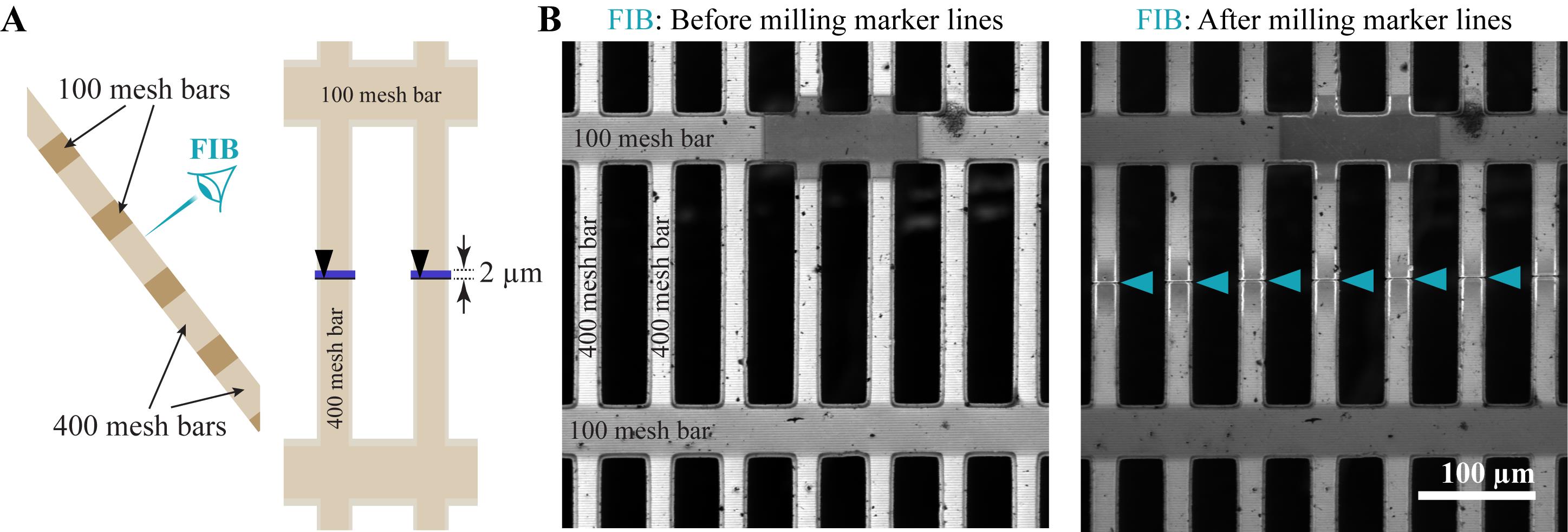
Figure 20. Milling of marker lines in trench milling orientation. (A) Schemes for the preparation of marker lines in trench milling orientation. The scheme on the left illustrates the location of grid bars with respect to the FIB imaging direction. The right scheme shows the milling patterns. Cross sections are indicated by blue rectangles and the milling directions by black arrowheads. (B) A 400 × 100 mesh grid before and after milling the marker lines (blue arrowheads) in the left and right panels, respectively. The FIB milling patterns are provided in the Supplementary Information.
B. Lift-out
1. Perform targeted trench milling and axial targeting of the target area as described in Part I, sections D and E. The only difference is that the final width (x-dimension) of the block containing the target area after trench milling is 50–55 μm.
Critical: Extending the width of the block (x-dimension with respect to FIB and SEM images) is vital for double-sided attachment. After detaching the lift-out block from the bulk sample, it must still be wide enough to bridge the gap between the two attachment sites. For double-sided attachment from the side using 400 × 100 mesh grids, this gap is about 40 μm wide. It is better to lift out a too-large block because you can always reduce its width. But once the lift-out block is too slim, the experiment fails.
C. Lift-in
1. Move the stage in lamella milling orientation (stage tilt = 15°) to the modified 400 × 100 mesh grid.
2. Precisely align the 100-mesh bars horizontally using the stage tilt. If the initial alignment error is larger than 10°, unload the receiver grid and adjust its orientation manually.
3. Find the coincidence point of FIB and SEM in the center of a grid rectangle between two marker lines.
4. Insert the needle with the lift-out block attached to it.
5. In the SEM, align the front edge of the lift-out block to the marker line on both grid bars.
6. Trim the lift-out block to fit into the gap between grid bars.
a. In the FIB, move the needle down until the lift-out block is 10 μm above the marker lines.
b. Trim the lift-out block horizontally to a width that is 200 nm wider than the gap between 400 mesh bars (Figure 21A) by milling two cross-sections on either side at 1 nA (z-dimension = 2 μm, milling direction toward the lift-out block).
Critical: Be cautious not to remove too much. If the lift-out block is a few hundred nanometers slimmer than the gap between 400 mesh bars, the experiment will fail.
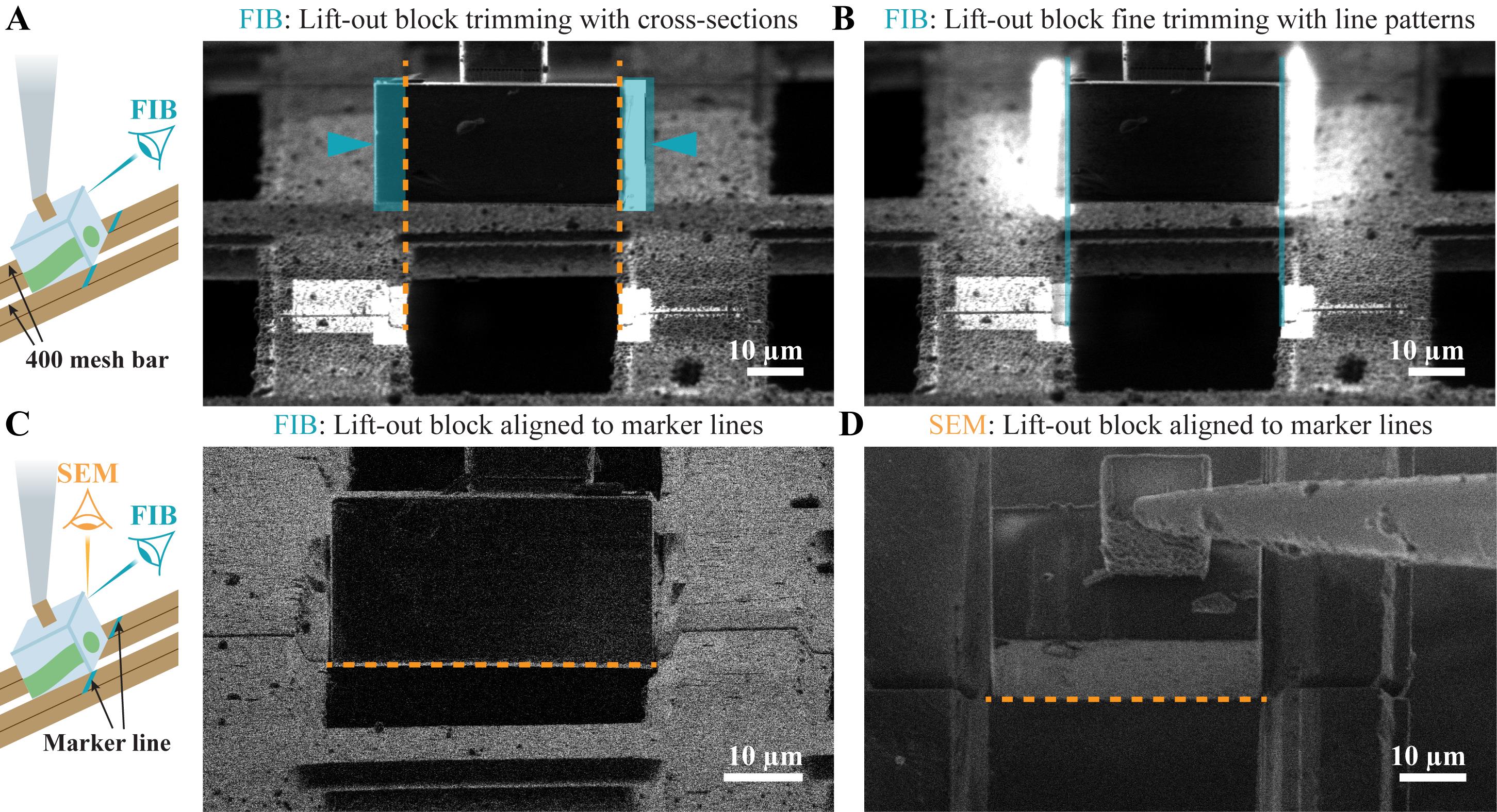
Figure 21. Trimming and alignment of the lift-out block for attachment from the side. The schemes on the left illustrate the location of the lift-out block with respect to marker lines and the FIB/SEM imaging directions. (A) Trimming of the lift-out block to be 200 nm wider than the gap between grid bars. Milling patterns are indicated by blue rectangles and milling directions by blue arrowheads. (B) If the lift-out block does not yet fit in between the bars, mill line patterns (blue lines) along the outer edge of grid bars starting from the marker line and ending above the lift-out block. (C) FIB image of the lift-out block’s lower edge aligned to the marker lines. (D) SEM image of the lift-out block’s lower edge aligned to the marker lines.
c. Center the lift-out block in the gap between the marker lines.
d. While imaging in the FIB, carefully move down the needle and check if the block fits between the grid bars until its lower edge aligns with the marker lines.
e. If not, move the needle 10 μm up and generate two vertical line patterns on either side of the lift-out block, starting from the marker line aligned to the outer edge of the grid bar, along the whole height of the lift-out block (Figure 21B).
f. Mill the line patterns (z-dimension = 3 μm) at 1 nA.
g. Repeat steps C6d–f until the lift-out block fits in between the grid bars and its lower edge aligns with the marker lines (Figure 21C).
7. In the SEM, check if the front edge is still aligned with the marker lines. If not, adjust the needle position (Figure 21D).
8. Generate the serial sections.
a. Define two vertical arrays of 6 cross-sections with xyz-dimensions of 2.5 × 0.5 × 4 μm every 250 nm. Place them along the interfaces between the grid bars and the lift-out block on either side of the grid bars. The lowest pattern on both sides aligns with the marker line. Set the milling direction away from the block (Figure 22A).
Critical: Set “multi pass” to 1 for the cross-sections used for redeposition milling.
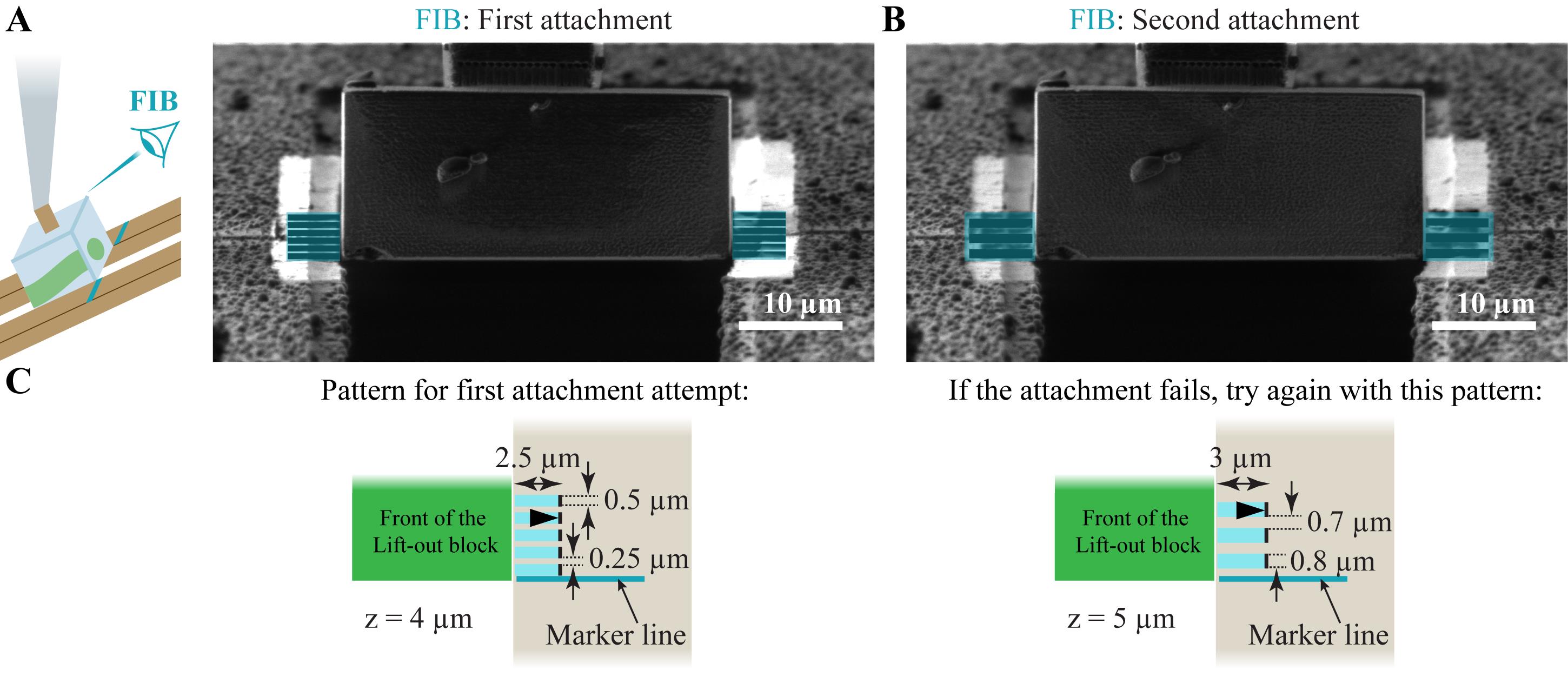
Figure 22. Attachment of serial lift-out sections from both sides. (A) Array of six cross-sections on either side, used for the attachment. The scheme on the left illustrates the location of the lift-out block with respect to marker lines and the FIB imaging direction. (B) If the attachment fails, a second array of fewer, wider, and deeper patterns can be milled. (C) Scheme of the cross-section arrays (“multi pass” set to 1) used for attachment for the first and second attempts in the left and right panels, respectively. The black arrowheads indicate the milling direction. The FIB milling patterns are provided in the Supplementary Information.
b. Mill the pattern arrays at 1 nA to attach the lift-out block on both sides.
Note: Move the needle 500 nm upward. You should see no movement or a movement of the entire grid. If only the lift-out block moves, the attachment was not successful.
c. (Optional) If the attachment was not successful, define two vertical arrays of three cross-sections with xyz-dimensions of 3 × 0.8 × 5 μm every 700 nm. Place them along the interfaces between the grid bars and the lift-out block on either side of the grid bars. The lowest pattern on both sides aligns with the marker line. Set the milling direction away from the block (Figure 22B). Mill at 1 nA.
d. Define a horizontal line pattern (z-dimension = 10 μm) that is 2 μm wider than the lift-out block and place it 4 μm higher than the lower edge of the lift-out block (line pattern I in Figure 23).
Note: The positioning of the line pattern above the lower edge of the lift-out block defines the section thickness. Thicker sections reduce the contextual information by resulting in fewer sections. Thinner sections are possible (2–3 μm), but that complicates the attachment and the subsequent sectioning and trimming step.
e. Define a pair of 4 μm wide horizontal line patterns (z-dimension = 20 μm). Place them on the first line pattern centered on the interfaces between the lift-out block and the grid bars on both sides (line patterns II in Figure 23).
Critical: During attachment, copper is sputtered on the sides of the lift-out block. This pair of line patterns is necessary to detach the section from the lift-out block on its sides.
f. Define a pair of vertical line patterns (z-dimension = 20 μm). Place them on the edge between the lift-out block and the grid bars on both sides, starting at the horizontal line patterns and ending 2 μm above the topmost patterns used for the attachment (line patterns III in Figure 23).
Critical: It is possible that the lift-out block becomes attached to the grid bars above the section. This second pair of line patterns is necessary to detach the lift-out block from the grid bars.
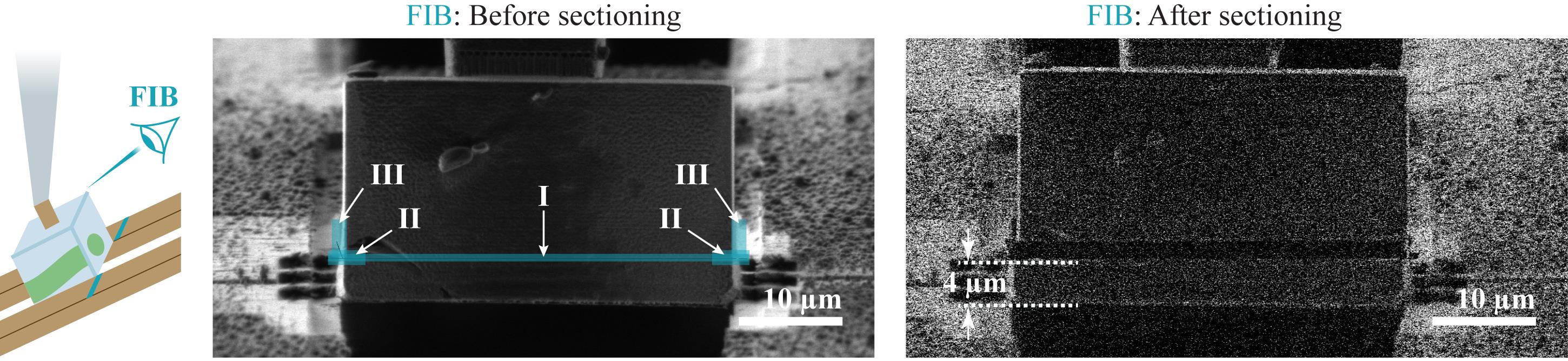
Figure 23. Sectioning of the lift-out block attached to the sides. The lift-out block before and after sectioning in the middle and right panels, respectively. The line patterns used for sectioning are indicated as blue lines in the middle panel. The scheme on the left illustrates the location of the lift-out block with respect to the FIB imaging direction. The white dashed lines in the right panel depict the section thickness. The FIB milling patterns are provided in Supplementary Information.
g. Mill all line patterns sequentially at 1 nA.
Note: Afterward, move the needle 500 nm upward. You should see movement of the needle and the remaining lift-out block. If nothing or the whole grid moves, the lift-out block is still attached to the section or the grid bars.
h. Retract the needle and move to the next attachment site.
9. Repeat step C8 until the whole lift-out block is sliced up.
D. Section trimming and fine milling
Perform section trimming and fine milling as described in Part II, sections D and E. Afterward, store the grid at liquid nitrogen temperatures.
Part IV. Serial lift-out with single-sided attachment
A. Prepare the lift-out session at room temperature
1. Load a half-moon grid into the FIB/SEM instrument.
Note: If you do not have half-moon grids, you can prepare grids with pins for single-sided attachment from a normal EM grid without support film as described in [1].
a. Clip the grid into a cartridge with a cutout for FIB milling. The half-moon grid must be clipped into the cartridge on the opposite side of the cutout.
b. If necessary, rotate the half-moon grid after clipping until it is on the opposite side of the cutout. Hold the cartridge on both sides with flat tweezers on a flat surface. Press with sharp tweezers against the edge of the clipped half-moon grid and rotate it relative to the cutout.
Critical: Do not touch the half-moon grid on its central front as this may bend the pins. If you deform the half-moon grid in the process of clipping or aligning, discard it and clip a new one. A bend half-moon grid as the receiver grid makes the experiment difficult or impossible.
c. Label the cartridge with two blue marks in the 3 and 9 o’clock positions, as well as a red mark at 6 o’clock, all with respect to the cutout 12 o’clock (Figure 24A).
Note: The marks will help you to orient the grid when loading it into the microscope.
d. Mount the clipped half-moon grid into the FIB shuttle. The cutout must face up, and the front edge with pins of the half-moon grid must be aligned horizontally (Figure 24B). Load the shuttle into the FIB/SEM instrument at room temperature.
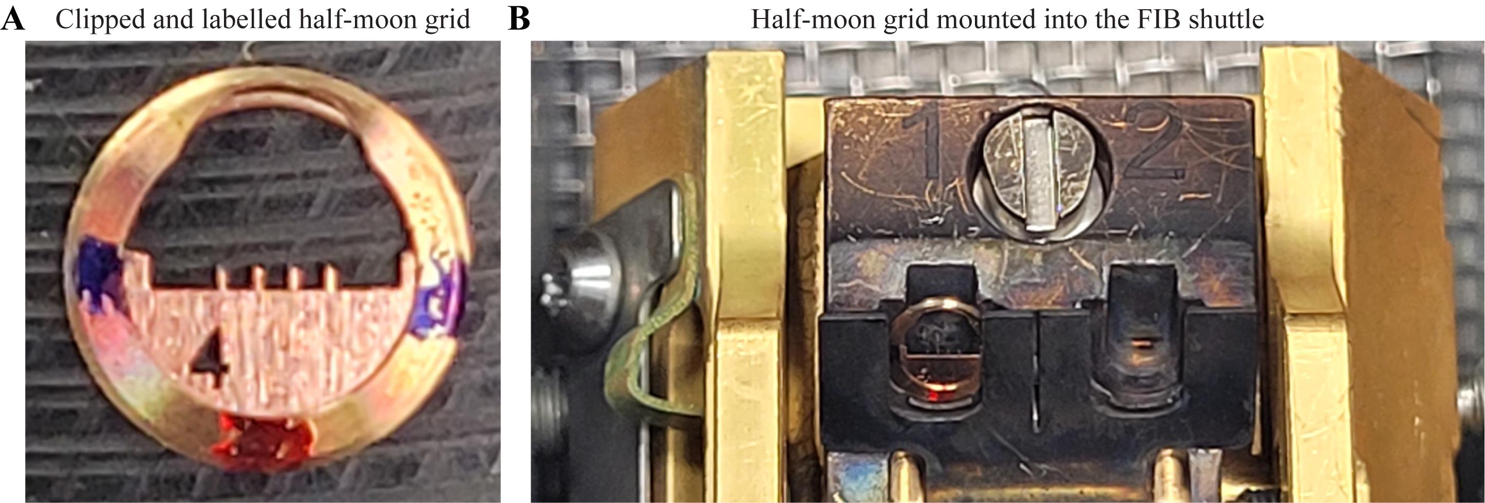
Figure 24. Labeling of the clipped half-moon grid and alignment in the FIB shuttle. (A) Markers on the cartridge of a clipped half-moon grid. (B) The half-moon grid mounted in the FIB shuttle.
2. Polish the bottom of the EasyLift needle.
a. Insert the needle.
b. Coarsely remove potential remnants of previous experiments at 5–30 nA.
c. Polish the bottom of the needle at 1 nA with a cross-section over the whole width of the needle bottom, with milling direction toward the needle. Set the z-dimension of the cross-section to the diameter of the needle at the tip.
d. Retract the needle.
3. Prepare and attach a copper adapter for the needle from the half-moon grid (Figure 25A).
a. Move the stage into trench milling orientation (stage tilt = 7°, relative rotation = 180°).
b. Find the coincidence point of FIB and SEM on the edge of the half-moon grid next to the pins (Figure 25B).
c. FIB-mill a cavity into the front edge of the grid using a cross-section with xyz-dimensions of 35 × 45 × 150 μm at 30 nA (Figure 25A, step I).
d. Mill a 20-μm-high cavity in y on the left side using a 5 × 20 × 150 μm cross-section (Figure 25A, step II), followed by a 35 × 5 × 200 μm trench in the back (Figure 25A, step III), both at 30 nA, creating the rough shape of a 30 × 15 μm copper adapter, which is attached to the grid on only one side (Figure 25C).
Note: The milling direction is always toward the copper adapter.
Critical: Take an FIB image and check if the copper adapter is detached on all three sides. If not, continue FIB milling until it is detached.
e. Rotate the stage into the lamella milling orientation and find the coincidence point of FIB and SEM on the precursor of the copper adapter.
f. Remove 10 μm from the top and bottom of the copper adapter using cross-sections with 35 × 10 × 30 μm in xyz at 30 nA (Figure 25D, steps IV and V).
g. Extend the top trench toward the right using a cross-section with 15 × 15 × 30 μm 30 nA (Figure 25D, step VI; Figure 25E).
Critical: The extension to the right is critical to allow the needle to get in contact with the top edge of the copper adapter. Otherwise, the needle may touch the surface of the grid before it comes in contact with the adapter.
h. Polish the top front of the copper adapter 1 nA (cross-section, xyz-dimension = 20 × 1.5 × 30 μm; Figure 25D, step VII).
i. With the stage in lamella milling orientation, insert the polished needle.
j. In the SEM, adjust the position of the needle so that the center of its tip aligns with the top edge of the copper adapter. This increases the surface for the redeposition (Figure 25F).
k. While continuously imaging with the FIB, move the needle down in z until it is in contact with the upper surface of the copper adapter.
l. Define a horizontal array of cross-sections with xyz-dimensions of 0.5 × 2.5 × 4 μm every 250 nm and place it along the interface between needle and adapter on the adapter with the milling direction away from the needle (Figure 25H).
Critical: Set “multi pass” to 1 for the cross-sections used for redeposition milling.
m. Mill the pattern array at 1 nA to attach the needle to the copper adapter (Figure 25G, step VIII).
Note: Move the needle 500 nm upward. You should see no movement or a movement of the entire grid. If only the needle moves, the attachment was not successful.
n. Detach the copper adapter on the remaining side. Use a cross-section with xz-dimension 5 × 30 μm over the whole height of the adapter milled at 5 nA (milling direction toward the adapter), resulting in a final adapter width of 15–20 μm (Figure 25G, step IX; Figure 25I).
Note: Single-sided attached lamellae are not as stable as double-sided attached lamellae. They tend to bend (see below in section E). This tendency is reduced if the width of the lift-out block is kept as small as possible, minimizing the distance between the attachment site and the outer edge of the lamella later. The width of the copper adapter must be smaller than the width of the lift-out block. The width of the copper adapter can be adjusted in this step by the position of the cross-section that detaches the adapter from the bulk grid.
o. If not yet done, polish the lower edge of the copper adapter at 1 nA (cross-section, yz-dimensions: 1.5 × 30 μm over the whole width of the adapter, milling direction toward the adapter).
Note: This can be done when the system is cooled down right before the lift-out experiment starts.
p. Retract the needle.
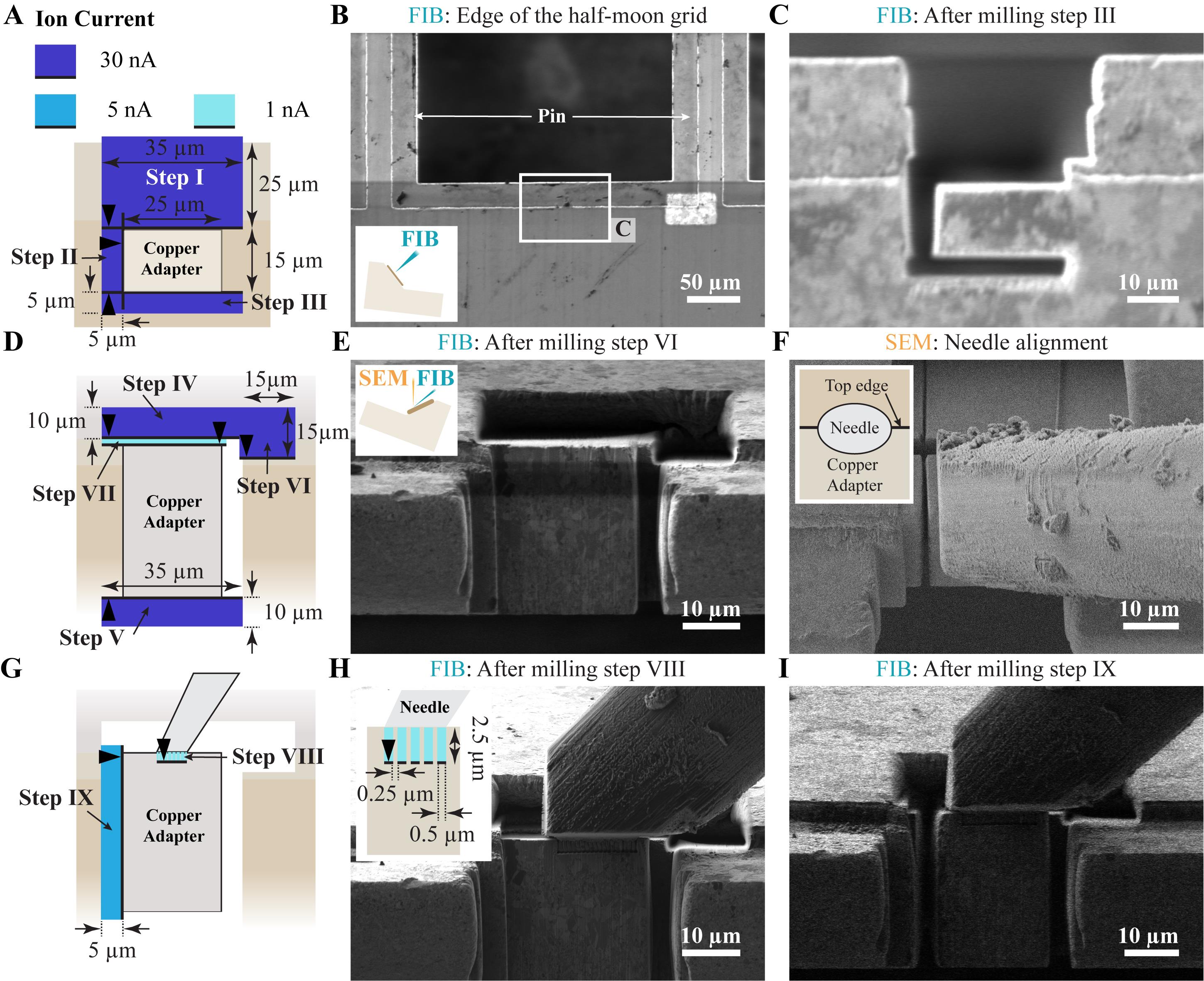
Figure 25. Preparation of a copper adapter from a half-moon grid. (A) Scheme of the first set of patterns used to mill the rough shape of the copper adapter with the stage in trench milling orientation. (B, C) Milling steps in trench milling orientation. (B) Edge of the half-moon grid between two pins. The inset illustrates the shuttle in trench milling orientation with respect to the FIB imaging direction. (C) FIB image after milling the rough shape of the copper adapter. (D–I) Milling steps in lamella milling orientation. (D) Scheme of the second set of patterns used to prepare the needle attachment site with the stage in lamella milling orientation. (E) FIB image after milling the needle attachment site. The inset illustrates the shuttle in lamella milling orientation with respect to the FIB/SEM imaging directions. (F) SEM image of the needle aligned above the copper adapter. The inset shows how the center of the needle bottom is positioned above the top edge of the copper adapter. (G) Scheme of the third set of patterns required to attach the needle and detach the copper adapter from the grid milled in lamella milling orientation. (H) Attachment of the needle to the copper adapter. The inset illustrates the dimensions of the used cross-section patterns (“multi pass” set to 1). (I) FIB image after detaching the copper adapter from the half-moon grid. In (A), (D), (G), and (H), black arrowheads indicate the milling directions of the cross-sections. The FIB milling patterns are provided in Supplementary Information.
4. Mill marker lines into the front edges of pins for the alignment of the lift-out block.
a. In the FIB, center the tip of a pin in trench milling orientation.
b. Align the pin vertically by adjusting the stage rotation.
c. Define cross-sections with xyz-dimensions of 10 × 2 × 12 μm (milling direction top to bottom) and place them on the edge of the pin at the transition to its round tip on both sides (Figure 26).
d. Mill the marker lines at 15 nA.
e. Repeat this for all pins.
f. Store the modified half-moon receiver grid until it is used for a lift-out experiment.
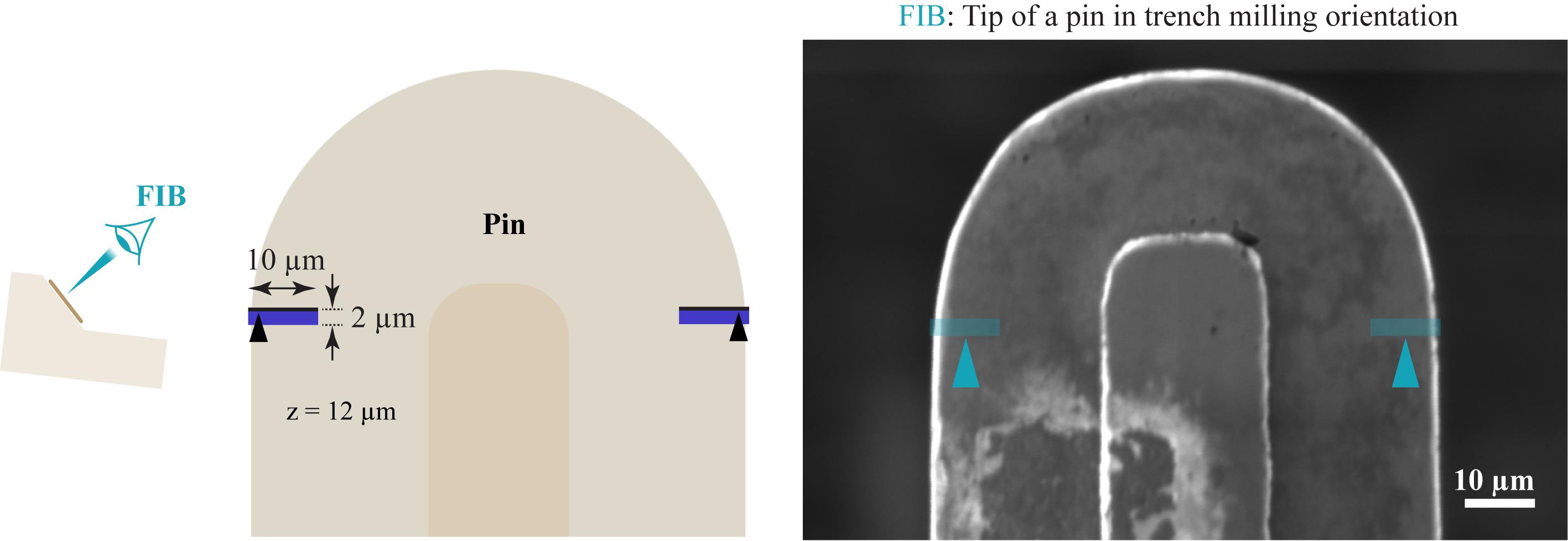
Figure 26. Marker lines for half-moon grids. The scheme on the left illustrates the stage in trench milling orientation with respect to the FIB imaging direction. The scheme in the middle and the FIB image on the right show the tip of a pin. The cross-sections used to mill marker lines are depicted as blue rectangles. The milling direction is indicated by arrowheads. The FIB milling patterns are provided in Supplementary Information.
B. Lift-out
1. Load the modified half-moon receiver grid and the sample for lift-out into the FIB/SEM instrument.
a. Mount the modified receiver grid into the FIB shuttle with the loading station at room temperature. Make sure the cutout for FIB milling is oriented on top, and the front edge of the half-moon grid is oriented horizontally. Fix the grid in the shuttle by tightening the screw.
Note: Orienting the receiver grid is much easier at room temperature.
b. Cool down the loading station.
c. Loosen the screw of the shuttle and load the lift-out sample into the shuttle.
d. Load both grids into the cooled FIB/SEM instrument after fixing them in the shuttle.
e. While imaging in the FIB, precisely align the edge of the receiver grid horizontally using the stage tilt.
Critical: If the alignment error is higher than 10°, unload and manually adjust the receiver grid orientation before reloading.
2. Do targeted trench milling and axial targeting as described in part I, sections D and E. The only difference is that the final width (x-dimension) of the block containing the target area is 25–30 μm after trench milling.
Critical: Single-sided attached lamellae are not as stable as double-sided attached lamellae. They tend to bend (see below in section D). This tendency is reduced if the width of the lamella relative to the attachment site is minimized and, therefore, if the width of the lift-out block is kept as small as possible.
C. Lift-in
1. Move to the half-moon grid with the stage in lamella milling orientation (stage tilt = 15°).
2. Find the coincidence point of FIB and SEM on a marker line at the edge of a pin.
3. Insert the needle with the lift-out block attached to it.
4. In the SEM, align the front edge of the lift-out block to the marker line with a 2 μm gap to the pin.
5. While imaging in the FIB, move down the needle until its lower edge is aligned with the marker line (Figure 27A).
6. In the SEM, check if the front edge is still aligned with the marker line. If not, adjust the needle position.
7. In the SEM, move the needle toward the pin until the lift-out block touches the pin.
8. Generate the serial sections:
a. Define a vertical array of six cross-sections with xyz-dimensions of 2.5 × 0.5 × 4 μm every 250 nm. Place them along the interfaces between the pin and the lift-out block on the pin. The lowest pattern aligns with the marker line. Set the milling direction away from the block (Figure 27B).
b. Mill the pattern array at 1 nA to attach the lift-out block on the side.
Note: Move the needle 500 nm upward. You should see no movement or a movement of the entire grid. If only the lift-out block moves, the attachment was not successful.
c. (Optional) If the attachment was not successful, define a vertical array of three cross-sections with xyz-dimensions of 3 × 0.8 × 5 μm every 700 nm. Place it along the interfaces between the pin and the lift-out block. The lowest pattern aligns with the marker line (Figure 27D). Mill at 1 nA.
d. Define a horizontal line pattern (z-dimension = 10 μm) that is 2 μm wider than the lift-out block and place it 4 μm higher than the lower edge of the lift-out block (line pattern I in Figure 27C).
Note: The positioning of the line pattern above the lower edge of the lift-out block defines the section thickness. Thicker sections reduce the contextual information by resulting in fewer sections. Thinner sections are possible (2–3 μm), but that complicates the attachment and the subsequent section trimming step.
e. Define a second horizontal line pattern (z-dimension = 20 μm) that is 4 μm wide. Place it on the first line pattern centered on the interface between the lift-out block and the pin (line pattern II in Figure 27C).
Critical: During the attachment, copper is sputtered on the side of the lift-out block. This second line pattern is necessary to detach the section from the lift-out block.
f. Define a vertical line pattern (z-dimension = 20 μm). Place it on the edge between the lift-out block and the pin, starting at the horizontal line patterns and ending 2 μm above the topmost pattern used for the attachment (line pattern III in Figure 27C).
Critical: It is possible that the lift-out block becomes attached to the pin above the section. This third line pattern is necessary to detach the lift-out block from the pin.
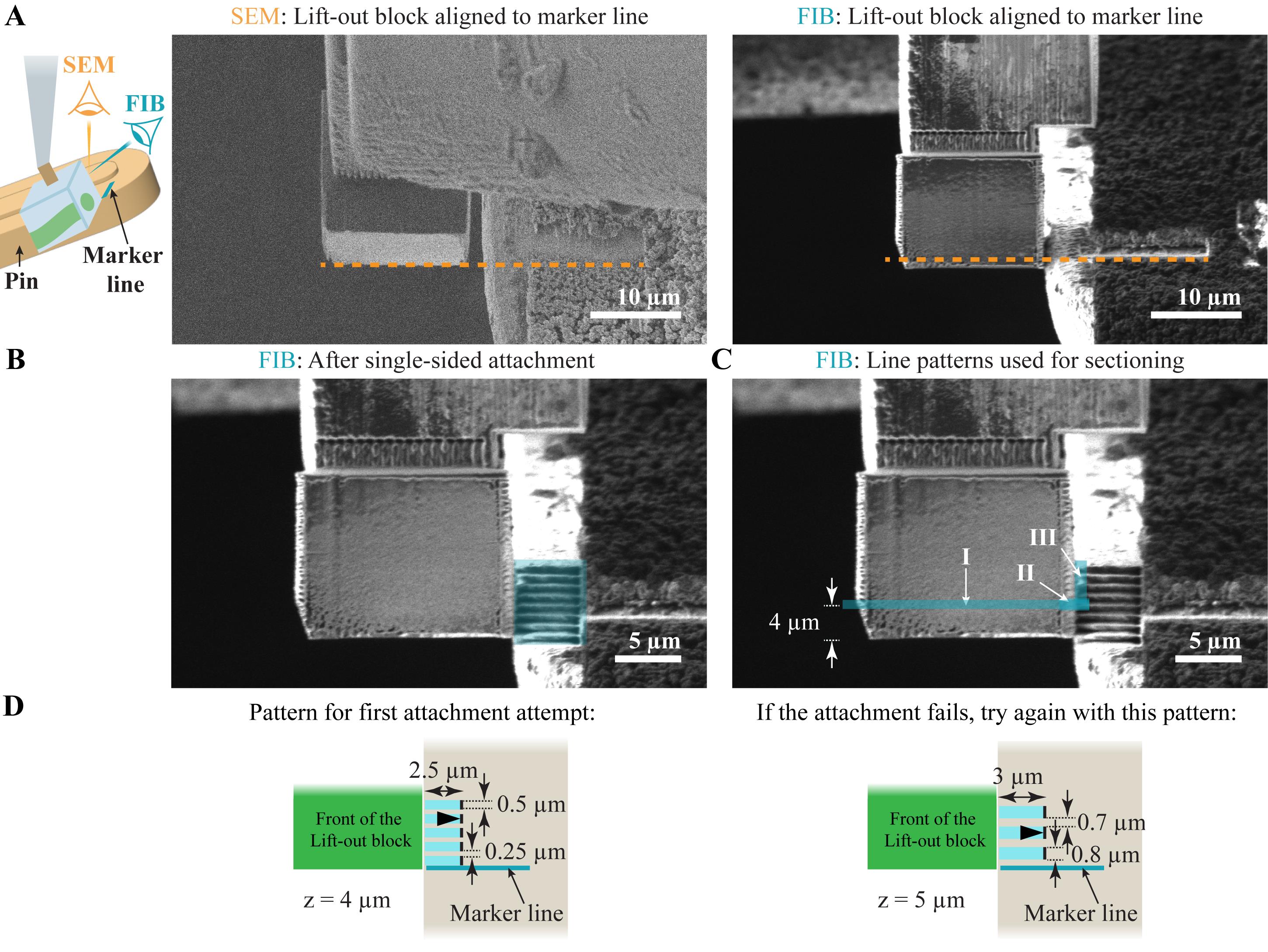
Figure 27. Alignment, attachment, and sectioning of the lift-out block for single-sided attachment. (A) SEM and FIB images of the lift-out block aligned to the marker line, shown in the left and right panels, respectively. The orange dashed line indicates the alignment to the marker line. The scheme on the left illustrates the location of the lift-out block with respect to the pin, marker lines, and the FIB/SEM imaging directions. (B) FIB image after the attachment from the side. (C) Line patterns for the sectioning of the lift-out block, indicated by blue lines. (D) Scheme of the cross-section arrays (“multi pass” set to 1) used for attachment for the first and second attempts in the left and right panels, respectively. The black arrowheads indicate the milling direction. The FIB milling patterns are provided in the Supplementary Information.
g. Mill all line patterns sequentially at 1 nA.
Note: Afterward, move the needle 500 nm upward. You should see movement of the needle and the remaining lift-out block. If nothing or the whole grid moves, the lift-out block is still attached to the section or the pin.
h. Retract the needle and move to the next attachment site.
9. Repeat step B8 until the whole lift-out block is sliced up.
D. Trim the sections
1. Record top-view images of every section with the int-FLM with the stage in trench milling orientation.
a. Use the reflected light channel to focus on the section.
b. Record a z-stack with reflected light and cellular autofluorescence channel as used for targeted trench milling (bin = 4, 10 z-slices, z-step = 1 μm).
2. Identify sections that do not contain the target area based on the int-FLM top views. These sections can be skipped in the subsequent steps (Figure 28A).
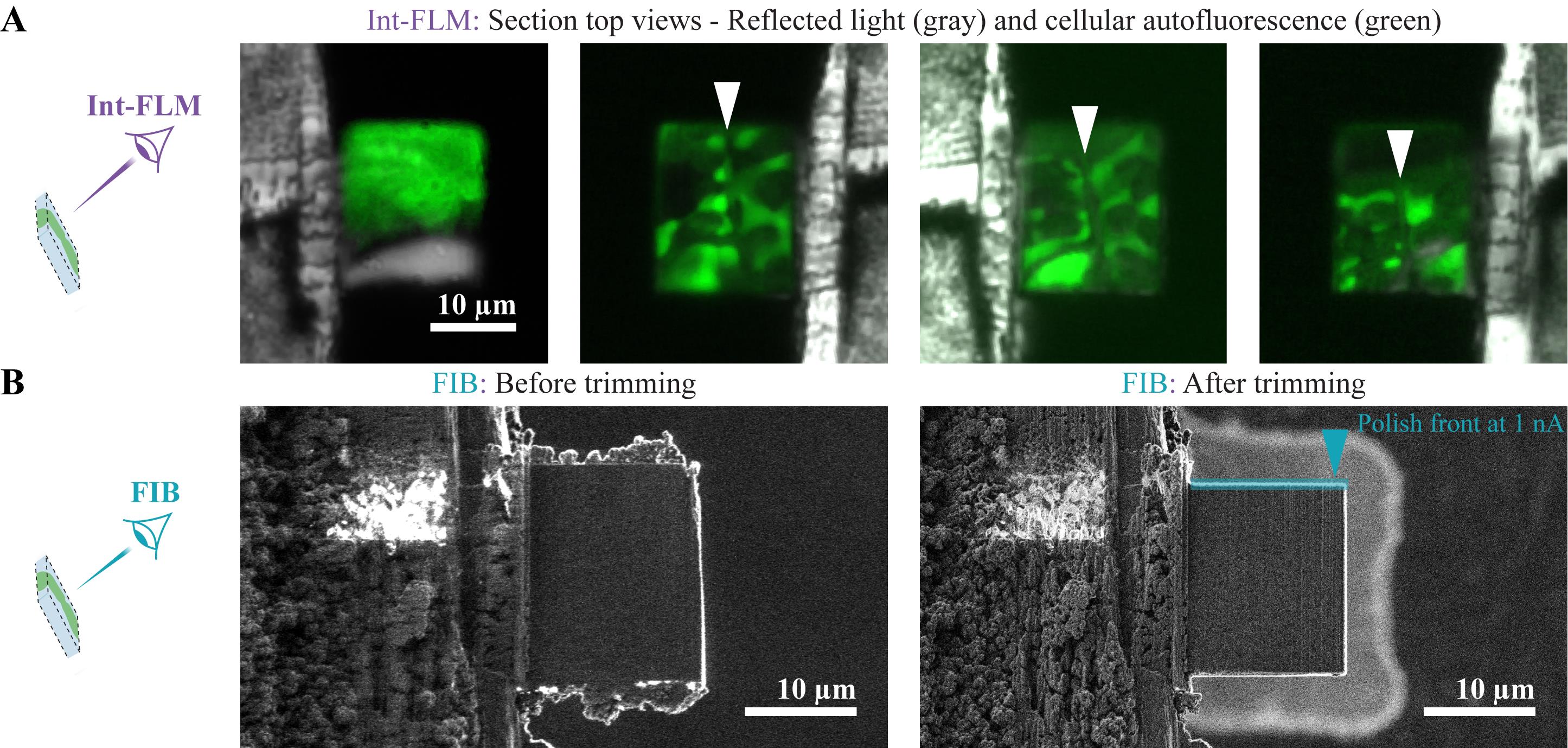
Figure 28. Trimming of single-sided attached serial lift-out sections. The schemes on the left illustrate the location of the section with respect to the int-FLM and FIB imaging direction. (A) Top views recorded with the int-FLM of four successive serial lift-out sections showing the reflected light channel (gray) and cellular autofluorescence (green). The junction between cells is only contained in three of them, as indicated by white arrowheads. (B) FIB images of a section recorded in trench milling orientation before and after trimming in the left and right panels, respectively. Afterward, the top front is polished at 1 nA. The milling pattern is indicated by a blue rectangle and the milling direction by a blue arrowhead. The FIB milling patterns are provided in Supplementary Information.
3. For sections that contain the target area, identify the regions of the sections that do not contain the material of interest based on the int-FLM top views.
4. Apply a layer of metal-organic platinum by opening the GIS 15 s in trench milling orientation at the GIS working distance in z.
5. For every section, remove material above and below the target area as well as on the side opposite to the attachment site with the stage in trench milling orientation. Use cross-sections (z-dimension = 1 μm) milled at 3 nA with the milling direction toward the target area (Figure 28B).
6. Polish the top front at 1 nA (cross-sections, z-dimension = 2 μm).
Critical: During trimming, at least 1–2 μm should be removed from the top edge. This surface was constantly exposed by the FIB during lift-out, lift-in, and sectioning. Thus, it is damaged and uneven.
7. Open the GIS in trench milling and lamella milling orientation for 15 s and 3 × 20 s, respectively, both at a GIS working distance.
Note: The trimming minimizes the size of the lamella, which makes fine milling faster and generates smooth surfaces covered with a thick, homogeneous layer of metal-organic platinum, which is key to obtaining homogeneously thin lamellae.
E. Thin the sections by FIB milling
1. Remove the top and bottom of the section over its whole width at 1 nA using cross-sections (top z-dimension = 5–6 μm, bottom z-dimension = 2 μm, vertical distance between patterns = 2 μm; similar to Figure 19A).
Note: The section’s top layer is composed of metal-organic platinum and requires longer milling times.
2. Thin the lamella to 1.5 μm at 0.3 nA using cross-sections (z-dimension = 2 μm, milling direction toward the center of the lamella).
3. Define two rectangle patterns with a vertical distance of 200 nm, but leave a 1.5 × 1.5 μm block opposite to the attachment site (Figure 29A).
Critical: This block prevents the lamella from curling during fine milling.
4. Mill the rectangle patterns in parallel at 50 pA.
5. Switch to an ion current of 30 pA. Tilt the stage to 14° and 15.5–16° and polish your lamella only from below and the top, respectively.
6. (Optional) Sputter a thin layer of metallic platinum on your sample (U = 1 kV, I = 10 mA, p = 0.2 mbar, t = 2–4 s).
7. Unload the sample and store it at liquid nitrogen temperatures until it is imaged in a transmission electron microscope.

Figure 29. Fine milling of single-sided attached sections. (A) Single-sided attached lamella before and after fine milling in the middle and right panels, respectively. The milling patterns are indicated in blue rectangles in the middle panel and the milling directions by blue arrowheads. A 1.5 × 1.5 μm block opposite to the attachment site is left to prevent curling of the lamella. The left panel illustrates the location of the lamella with respect to the FIB imaging direction. (B) Single-sided attached lamellae, which bend after fine milling. The FIB milling patterns are provided in Supplementary Information.
Part V. Workflow for in-carrier high-pressure frozen samples
A. In-carrier high-pressure freezing
1. Clean 3 mm type-A and type-B HPF carriers the day before high-pressure freezing.
a. Incubate carriers overnight in a 15 mL Falcon tube with cleaning solution.
b. Wash carriers 3× with ddH2O and 3× with acetone.
c. Dry carriers on filter paper.
2. Coat type-B carriers with cetyl palmitate.
Note: Work under a fume hood.
a. Dip the type-B carriers (one 300 μm cavity and one flat side), one at a time, with tweezers into cetyl palmitate solution.
b. Remove excess liquid by shaking it off and pushing the side of the carriers against filter paper.
c. Dry carriers on filter paper with the flat side facing up.
3. Label the rim of type-A carriers on the side with the 100 μm deep well with a red and a black mark in the 6 and 12 o’clock positions, respectively.
Notes:
1. Use magnifying glasses or binocular microscopes to discern the side with the 100 μm from the 200 μm well.
2. The label helps to identify the sample-containing side of the carrier and can be used to orient the carrier when loading it into the FIB/SEM instrument.
4. Prepare the high-pressure freezer and test the system.
a. Cool down the high-pressure freezer and the sample container. Insert the sample container and wait for the system status to change to ready.
b. Freeze two “test shots” only with two half cylinders and a middle plate without HPF carriers.
5. Place a type-A carrier with the marked side facing up on a filter paper.
6. Add 2 μL of freezing buffer into the 100 μm well and distribute it with the pipette tip.
7. Pick up a small patch of a Physcomitrium patens protonemata from a plate and place it in the droplet in the center of the carrier.
Critical: Try not to squeeze the tissue with tweezers. This will damage the cells. Lift the tissues with the tip of a single leg of the tweezers.
8. Remove air bubbles by poking them with sharp tweezers.
Critical: Air bubbles in the sample will first be compressed upon high-pressure freezing but expand again when the freezing chamber is depressurized. This can induce cracks in your sample, which makes subsequent steps difficult or even impossible.
9. Remove excess buffer until its meniscus almost vanishes. For large volumes, use 2 × 0.5 cm filter paper pieces. For small volumes, stick closed tweezers into the buffer, open them, and take them out of the buffer.
Critical: The convex buffer meniscus must almost but not entirely vanish. If the meniscus becomes concave, you will create a large air inclusion when you place the flat side of the type-B carrier on top, which will cause freezing problems.
10. Place a cetyl palmitate–coated 3 mm type-B carrier with the flat side down on top and squeeze the sandwich together.
11. Remove excess buffer with a 2 × 0.5 mm piece of filter paper at the gap between carriers.
12. Place the carrier sandwich in the plastic pieces of the high-pressure freezer.
13. Squeeze the sandwich for 10 s with the back side of tweezers.
14. Freeze the sample.
15. Recover the sample containing type-A carriers by separating them from the type-B carriers.
Pause point: Store samples in grid boxes cooled by liquid nitrogen until use.
B. Sample screening and targeted trench milling
Note: The 3 mm HPF carriers have a slightly smaller diameter than grids clipped into cartridges. The commercial Leica SP8 shuttles are designed for cartridges. Thus, 3 mm HPF carriers cannot be screened in the FLM as described for the waffle workflow in the previous sections. Record tile images with the int-FLM instead. This is sufficient to find target areas. The tissue is overall better preserved because damage due to compression by grid bars or multiple cell layers per grid square is omitted by in-carrier high-pressure freezing.
1. Load an in-carrier frozen sample and a clipped receiver grid (see previous sections) into a cooled cryo-FIB/SEM instrument with int-FLM.
Critical: Check at room temperature if your FIB shuttle holds both the 3 mm carrier and the receiver grid. On some shuttles, the receiver grid falls out because the 3 mm carrier is thicker than the cartridge. If the receiver grid falls out, first, load only the carrier and do the lift-out. Then, unload the 3 mm carrier and load the receiver grid.
2. Remove ice contamination with the FIB (see Figure 3).
3. (Optional) Sputter coat the sample (p = 0.1 mbar, U = 1 kV, I = 10–30 mA, t = 15–30 s).
Note: The resulting Pt layer prevents charging, especially for thicker samples, which improves the quality of FIB and SEM images.
4. Apply a layer of metal-organic platinum by opening the GIS for 45 s in trench milling orientation at the GIS working distance in z.
5. With the stage in trench milling orientation, find the coincidence point of SEM and FIB in the center of the carrier.
6. Mill a marker (cross-section, I = 3 nA, z = 0.5 μm, Figure 30A).
Note: An asymmetric marker can be beneficial if FIB and int-FLM images are rotated with respect to one another. Here, we used an 8 × 8 μm square with a 6 × 16 μm rectangle aligned with their upper edges at a distance of 8 μm.
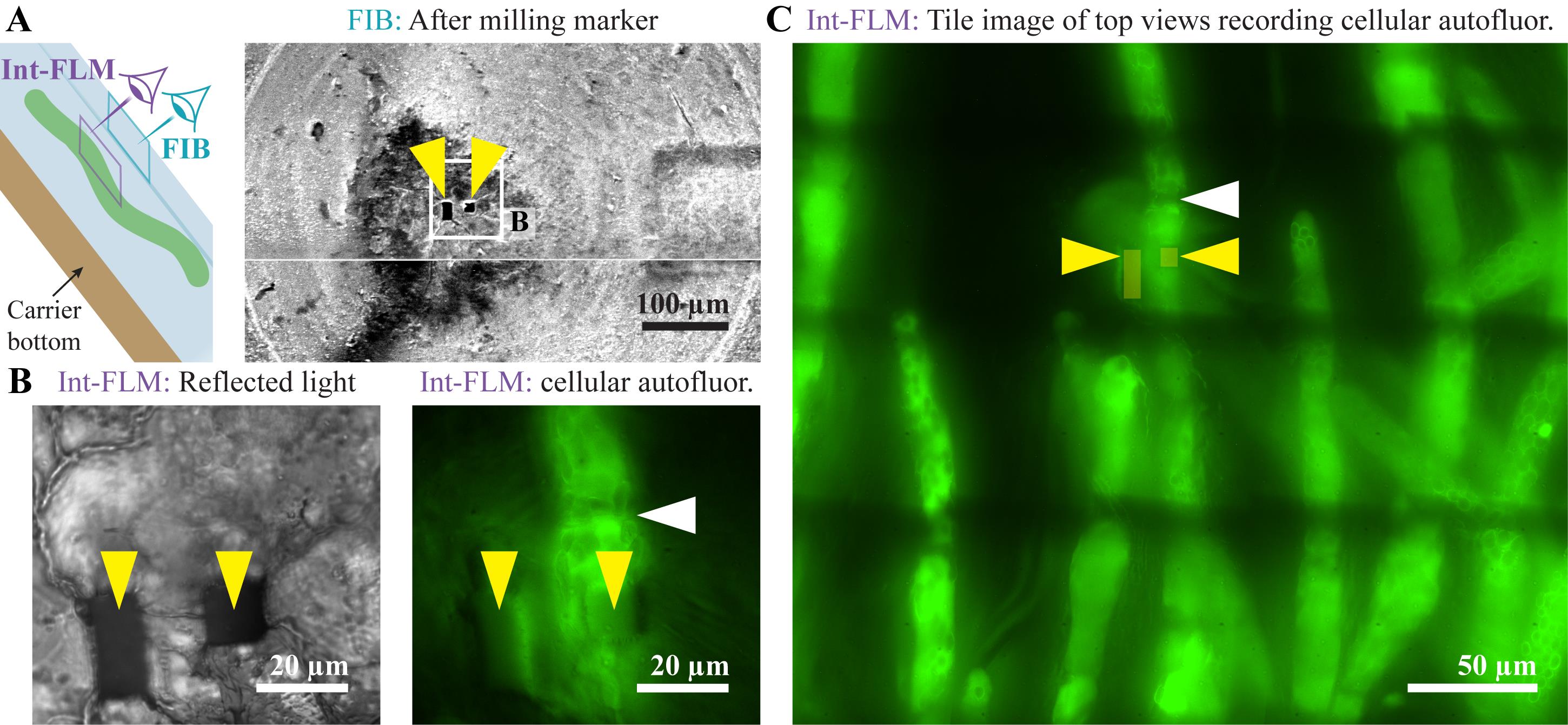
Figure 30. Screening of in-carrier frozen samples using the int-FLM. (A) In-carrier frozen sample with an asymmetric marker pattern milled in the center of the sample. The scheme on the left illustrates the location of the sample with respect to the FIB and int-FLM imaging direction. (B) Top views recorded with the int-FLM. The reflected light and cellular autofluorescence channels are depicted in the left and right panels, respectively. (C) Tile montage of Int-FLM top views recording cellular autofluorescence. Marker holes are indicated by yellow arrowheads, and a junction between cells is indicated by a white arrowhead.
7. Use the int-FLM to screen the sample by recording tile images of top views.
a. Focus the int-FLM on the sample surface and locate the marker pattern (Figure 30B).
Note: This is easiest using a reflected light channel (excitation: 470 nm ± 10 nm; no emission filter).
b. Record tile images covering 500–1,000 μm2 as z-stacks with 5–10 z-steps and a step size of 5–10 μm using the reflected light and cellular autofluorescence (excitation: 470 nm ± 10 nm; emission filter: 515 nm ± 15 nm; Figure 30C).
Critical: Keep the laser power as low as possible while still being able to identify your target area. Too-high laser power can devitrify your sample.
Note: Dependent on the int-FLM system, the imaged area, and the z-stack size, this can take hours.
c. Identify a potential target area, move the stage there, and record a z-stack (Figure 30B; bin = 4, 20–25 z-slices, z-step = 1 μm).
Note: Ideally, target areas should be located close to the sample surface, which can be estimated in int-FLM z-stacks. Lift-out on targets that are located tens of micrometers below the sample surface is challenging. The closer the target area is located to the surface of the sample, the more accessible it is for the lift-out.
8. Targeted trench milling was performed as described in the waffle workflow with two important differences:
a. Set the z-dimension of the milling patterns to 1–1.5 μm.
Critical: If you mill for too long, which is determined by the patterns’ z-dimension, you will reach the metal surface at the bottom. This will sputter metal from the carrier onto the front of the block containing the target area, which makes the generation of a smooth front very difficult.
b. Adjust the xy-dimension of the trench milling patterns dependent on the attachment strategy for the lift-in as described in previous sections.
Notes:
1. For the double-sided attachment, the width of the lift-out block (x-dimension with respect to FIB and SEM images) must be wide enough to bridge the gap between attachment sites.
2. For the single-sided attachment, it is beneficial if the width of the lift-out block is kept at a minimum, while the depth is increased (y-dimension with respect to FIB images recorded with the stage in trench milling orientation). This increases the area for the attachment and may prevent lamella bending.
C. Lift-out
Critical: To detach the lift-out block in in-carrier frozen samples, it is not enough to detach it on all four sides in trench milling orientation, as is the case for waffle samples. It requires a FIB milled “undercut” in lamella milling orientation to detach the lift-out block on the bottom from the bulk sample.
1. Determine the axial location of the target area using SEM block-face imaging (Figure 31B) or FIB-view imaging with the integrated FLM (Figure 31C).
Critical: The axial localization is crucial. In-carrier HPF samples are substantially thicker than waffle samples. This step helps you to make sure you lift out your whole target area and not much less or more.
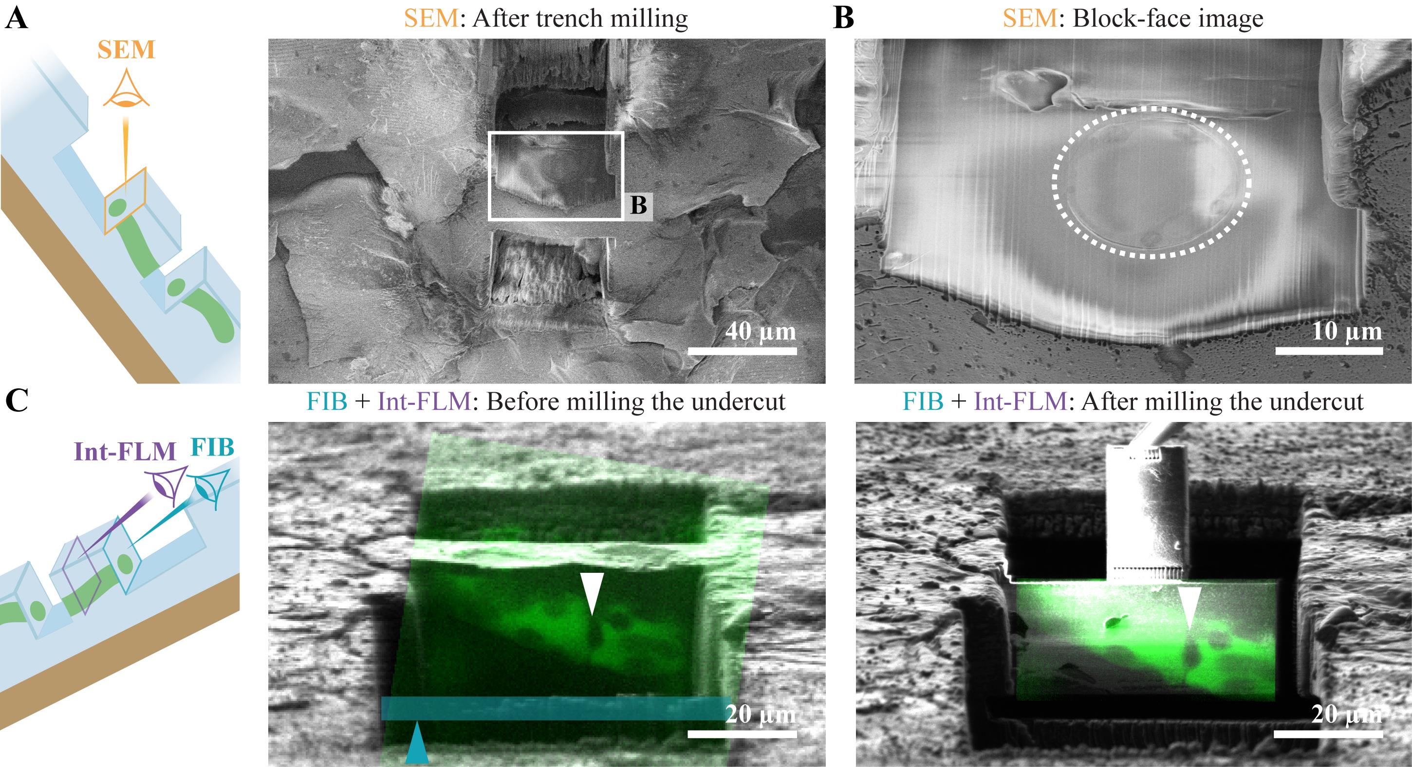
Figure 31. Lateral targeting and undercut for lift-out on in-carrier frozen samples. The schemes on the left illustrate the location of the sample with respect to the SEM, int-FLM, and FIB imaging directions. (A) SEM image of an in-carrier frozen sample after trench milling. (B) SEM block-face image of the surface exposed through trench milling. The lateral location of a cell is indicated by a dashed white line. (C) Overlay of FIB (gray) and FIB-view images recorded with the int-FLM (cellular autofluorescence in green) before and after milling the undercut. The undercut milling pattern is indicated by a blue rectangle, the milling direction by a blue arrowhead, and the junction between cells by white arrowheads.
2. Apply a layer of metal-organic platinum.
a. Rotate the stage into lamella milling orientation and move the stage to the GIS working distance.
b. Lift-out option I: from the side similar to ([1]): open the GIS for 20 s.
c. Lift-out option II: from the top: open the GIS for 3 × 30 s.
Critical: If you perform the lift-out in lamella milling orientation, the front of the block containing the target area will be constantly exposed by imaging with the FIB. Thus, it needs a thicker protective layer.
3. Create a cross-section for the “undercut” over the whole width of the block containing the target area with yz-dimensions of 3 × 4 μm and milling direction bottom to top.
Critical: The required z-dimension of the pattern depends on the thickness of the lift-out block in the direction of the optical axis of the FIB. It may need adjustment if the block is thicker than 30 μm.
4. Place the undercut pattern below the target area based on its z-location and mill it at 3 nA.
5. Proceed with the lift-out as described in Part II, step B3 or 4.
D. Lift-in, section trimming, and fine milling
Perform lift-in, section trimming, and fine milling as described in the previous sections, dependent on the chosen attachment strategy:
Option 1: Part II, sections C–E.
Option 2: Part III, sections C and D.
Option 3: Part IV, sections C–E.
Data analysis
Data acquisition, examples of reconstructed tomograms, as well as workflows for data analysis and subtomogram averaging are described in [2] and [16].
Validation of protocol
We high-pressure-froze 45 P. patens samples (Figure 32A). In 21 of these samples (47%), we obtained lamellae with vitreous tissue. The HPF results are not consistent and sample-dependent. Sometimes, even within the same grid square, one lamella can be vitreous while another one, a few micrometers apart, is not. We tested the protocol on Nicotiana benthamiana trichomes, and not a single sample was vitreous (N = 10). At the same time, other users high-pressure-froze Caenorhabditis elegans L1 larvae with a success rate close to 100% (N > 20).
In total, we prepared 216 lamellae. Of 74 on-grid milled waffle lamellae, 80% survived the transfer into the TEM and could be imaged. A fraction of the non-imaged waffle lamellae, however, made the transfer, but not all material below them was removed by FIB milling. These “shadow lamellae” prevent cryo-ET data acquisition. For single-sided, double-sided attached lamellae from the side, and double-sided-attached lamellae from below, we prepared 31, 49, and 99 lamellae, of which 58%, 76%, and 90%, respectively, could be imaged (Figure 32B).
From data recorded on these lamellae, we recovered subnanometer structural details by subtomogram averaging as described in [2] and investigated the in situ architecture of plasmodesmata in P. patens [16]. Furthermore, we applied modified workflows to other plant tissues and species [2].
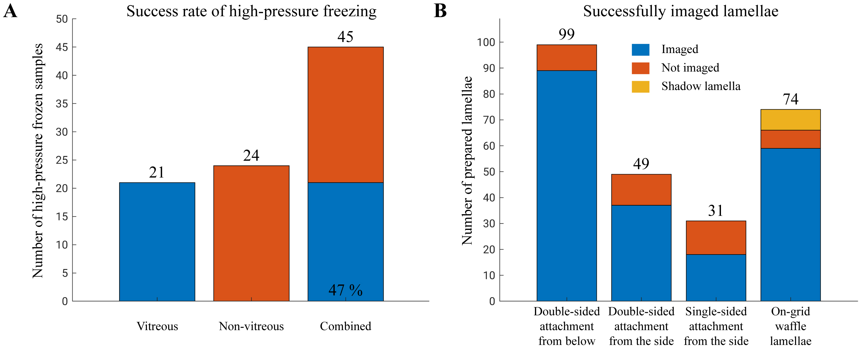
Figure 32. Success rates for high-pressure freezing and lamella preparation. (A) Success rate for high-pressure freezing for P. patens tissue. (B) Number of lamellae that were prepared compared to the number of imaged lamellae. For on-grid milled waffle lamellae, the fraction “Shadow lamella” indicates lamellae where not all material was removed below the lamella, which prevents the acquisition of cryo-ET data.
General notes and troubleshooting
General notes
1. Before using the FIB/SEM instrument, we recommend purging the gas injection system (GIS) and the integrated sputter coater to obtain consistent results when using them.
2. FIB and SEM imaging conditions: They are dependent on user preference and a compromise between seeing enough and not damaging the sample too much. We always detect secondary electrons with the Everhart–Thornley detector (ETD). For standard scanning (not block-face images), we prefer images with ~1,500 × 1,000 pixels with dwell times of 200–300 ns without line integrations, at U = 3 kV and I = 13 pA in the SEM and at U = 30 kV and I = 1.5–10 pA in the FIB. For imaging at ion currents larger than 50 pA, we use single scan snapshots with a dwell time of 100 ns and no line integrations. To document the experiment or for presentations/publications, we record images with 3,000 × 2,000 pixels, increase the exposure approximately 10×, reduce the dwell time (50–100 ns), and use several line integrations (10–20).
3. Scan rotation of FIB and SEM: We prefer a scan rotation of 180° for FIB and SEM. In this case, however, the int-FLM images recorded with the METEOR are rotated by 180° with respect to FIB images, and the needle of the lift-out system moves in positive x/y when you click negative x/y. Only movements in z appear correct. If the FIB/SEM scan rotation is set to zero, int-FLM and FIB images have the same rotation, x/y movements of the lift-out needle are not inverted, and the z-movements of the needle are inverted.
4. Orientation of the milling pattern: The orientation of the milling patterns is only correct at a scan rotation of 180°. Otherwise, all patterns must be rotated by 180°.
5. Stage tilts: All stage orientations, especially the stage tilts, described throughout the protocol (illustrated in Figure 2), are only valid for shuttles with a pretilt of 45°. For shuttles with different pretilt, all stage tilts must be adjusted.
6. The working distance of the gas injection system (GIS) and the thickness of the deposited layer may differ between FIB/SEM instruments and depend on the preset temperature of the GIS. You can roughly measure the GIS deposition rate by doing the following experiment:
a. Cool down the FIB/SEM instrument.
b. Load a holy carbon grid (e.g., Quantifoil R2/1 holy carbon 200 mesh copper grid) in trench milling orientation at a stage tilt of 20°.
c. Align the FIB optics on some contamination next to a hole.
d. Center a hole and save the position.
e. Take a long-exposure FIB image.
f. Measure the apparent vertical thickness of the carbon film in the FIB/SEM user interface without tilt correction.
g. Move the stage to the GIS deposition position and open the GIS for 20 s.
h. Go back to the hole, focus the SEM, run auto brightness/contrast, record an image, and measure the vertical thickness of the carbon film.
i. Repeat steps f–g approximately 10 times.
j. The corrected film thickness (tcorrected) depends on the measured thicknesses (tmeasured) and the stage tilt (αStage) according to the following equation:
tcorrected = tmeasured/sin(135° + αstage) = tcorrected/sin(155°)
Note: Here, the stage tilt was 20°.
Critical: This equation is only correct for the standard Thermo Fisher Scientific Scios/Aquilos FIB/SEM geometry and a shuttle with a pretilt of 45°.
k. Plot the corrected film thickness over the cumulative GIS deposition time (Figure 33A) and do a linear interpolation to estimate the deposition rate. In our case, the deposition rate is approximately 5 nm/s (Figure 33B). Hence, if we initially open the GIS for 45 s, a ~225-nm-thick layer of metal-organic platinum is applied onto the sample surface.
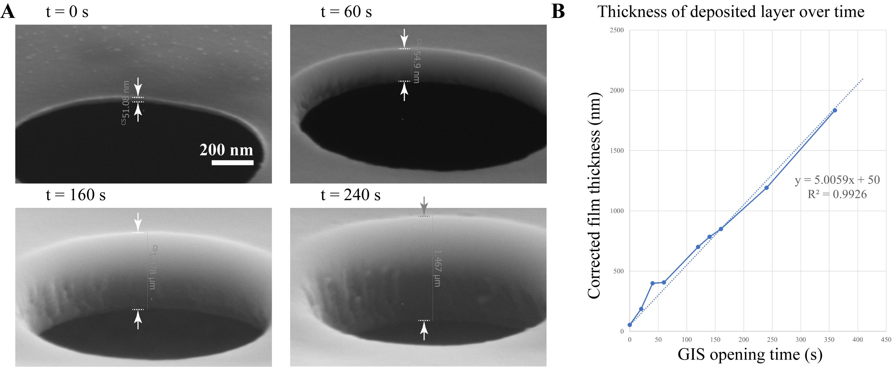
Figure 33. Estimating the deposition rate of the gas injection system (GIS). (A) Images of the apparent support film thickness at four different GIS opening times. (B) Corrected film thickness, plotted against the cumulative GIS opening time. The linear interpolation reveals that on the tested system, approximately 5 nm/s are deposited.
7. Types of milling patterns: Apart from the last fine milling step (at 50 and 30 pA), all milling patterns were regular cross-sections. While milling, they do not provide an immediate readout of what is happening, as is the case for rectangle patterns, but they deplete material faster and create smoother surfaces, which makes lamella milling faster and attachments easier.
8. Smooth attachment sites: The success rate of attachments by reposition milling is improved if the surfaces for attachment are smooth. Hence, all attachment surfaces were polished at 1 nA with cross-sections.
9. Milling patterns for redeposition milling: For cross-section patterns that were used to attach surfaces by redeposition milling, the “multi pass” number was set to 1, in contrast to cross-sections used to remove material, where the default “multi pass“ number was left at 4. Several passes remove material that was redeposited in the previous pass. In the case of redeposition milling, we rely on this redeposited material to weld surfaces together. Hence, we only allow a single pass.
10. Drift suppression: Switch on the drift suppression for all trench milling steps. Before you activate it, set the SEM magnification to 250×–1,000×. After activating drift suppression, center the green crosshair in the SEM channel roughly on the milling area. Especially for thick, not-conductive samples, like in-carrier frozen specimens, drift suppression reduces charging, which would otherwise deflect the FIB uncontrollably, damage the sample surface, and prevent milling of smooth trenches.
11. The z-thickness of patterns: The z-value of patterns defines their milling times and was optimized in this protocol for P. patens samples with a thickness of 25 μm. The thickness of waffle grids depends on the thickness of the grid bars. Thicker samples can be frozen in thicker grids (e.g., 50 μm thick slot or hole grids) to avoid squeezing damage. For different tissues or thicker grids, the milling times must be adjusted. For example, the Arabidopsis thaliana embryo sample described in [2] required 10× longer milling times than we used here.
12. Laser power for cryo-FLM: Keep the laser power as low as possible while still being able to see the target area. Too-high laser power can melt your sample.
13. FIB-view imaging with the int-FLM: This imaging mode is only possible when using a low NA objective with a working distance of approximately 10 mm. High NA objectives with short working distances would crash into the back of the shuttle before the sample is in focus.
14. Moving the lift-out needle: The EasyLift system used for the lift-out experiments can be moved in three modes. (i) Pressing the left mouse button either in the SEM or FIB channel and dragging the cursor into the desired direction or choosing the moving direction by clicking arrows in (ii) jog mode or (iii) step mode. In the jog mode, the arrow buttons can be continuously pressed, and the needle will move at the selected speed in the specified direction. In step mode, the needle moves upon clicking one step of the selected distance in the specified direction. For beginners, we recommend using the step mode. Click once to move the needle in a certain direction and wait until you see that the needle stops moving before you click the next time. If the scan speed is too slow or the system is lagging, you can crash the needle into your sample, which can damage both.
15. Moving direction of the needle: With a 180° scan rotation, using the xy-movement button results in an inverted response of the needle, i.e., if you press to the left, the needle moves to the right. Up and down in z, however, moves the needle in the apparently correct direction. With the scan rotation of 0°, z-movements are inverted, but the xy movements appear correct.
16. The stage tilt used for lift-in: Here, the lift-in was done at a stage tilt of 15°. It can be performed at lower or higher tilt angles. At lower tilt angles, however, the attachment sites might be hidden behind the rim of the cartridge, which makes lift-in impossible. To avoid this, attachment sites can be prepared closer to the lower edge of 400 × 100 mesh grids. But care must be taken that the stage of the TEM can still reach these sites. Attachment and fine milling at higher stage tilts can avoid this problem, but it might not be possible to acquire the full ±60° tilt range in a TEM starting from the effective zero tilt on the lamella. The lamella pretilt using a 45° shuttle is the stage tilt used for fine milling minus 7°.
17. Record movies: When you do the fine milling of lamellae using rectangular patterns, record a movie writing frames every 2–5 s. In case something goes wrong, the movies can help with troubleshooting.
18. Dimensions of lamellae: Apart from the final thickness of the lamella, it is also worth considering the width and depth with respect to the FIB imaging direction during fine milling. Here, we were aiming for 20 × 20 μm because a lamella of this dimension can contain a full cell junction. As a rule of thumb, however, the smaller a lamella is, the faster it can be thinned down, and the easier it is to obtain a homogeneously thin lamella. On the other hand, the lamella must be substantially larger than the desired field-of-view for cryo-ET data acquisition with enough space for at least one tracking area, ideally along the tilt axis of the used TEM.
19. Sputtering after fine milling: On our system, sputtering after fine milling introduced 5–15 nm Pt beads on the lamella surface. For us, they improve the motion correction of movies recorded in the TEM and tilt-series aligned with them, as fiducials result in better quality tomograms. Unfortunately, every sputter system behaves a bit differently and may not introduce fiducials at all. Therefore, the sputter settings for introducing fiducials must be tested and optimized for each individual FIB/SEM instrument.
20. How to avoid ice crystal contamination on lamellae: Lift-out lamellae, in particular, tend to accumulate ice contamination during transfers between microscopes. This is hard to completely avoid. It can be minimized if you work as fast as possible and use clean, fresh liquid nitrogen for (un)loading. When cooling down the loading stations, we pour the liquid nitrogen through a lint-free cloth to filter out ice contamination. If possible, work in a dry room.
Troubleshooting
1. Change the FIB aperture strip: The aperture strip regulating the ion current of the FIB is a consumable with limited lifetime. At the end of its lifetime, several problems can occur. An obvious problem is if the image at a certain current cannot be focused because the aperture is not round anymore. A less obvious problem is if the ion current on your sample is higher than indicated by the selected aperture because the hole has increased over time. This can burn your sample and make fine milling impossible. You can check the ion current that effectively reaches the sample while milling in the bottom left of the FIB/SEM user interface, where the measured “ion beam current” is displayed. In both cases, the aperture strip must be replaced.
2. The front after trench milling becomes uneven (Figure 34A): In this case, the applied layer of metal-organic platinum is probably too thin. Do not try to continue. Under these conditions, obtaining a homogeneously thin lamella is impossible (Figure 34B). Rotate the stage back into the trench milling orientation. Remove 1–2 μm of the old uneven front at 1 nA and apply a thicker protective layer with the GIS (i.e., open the GIS for a longer time) before you continue.
3. The detachment of a section failed: After milling the line pattern(s) for detachment, do the following check: Take a snapshot with the FIB, move the needle 500 nm up in z, and take another snapshot. You should only see that the needle with the remaining lift-out block moves up. If nothing moves or the whole grid moves up, the detachment failed. Increase the z-dimension of the lift-out pattern(s) and mill again.
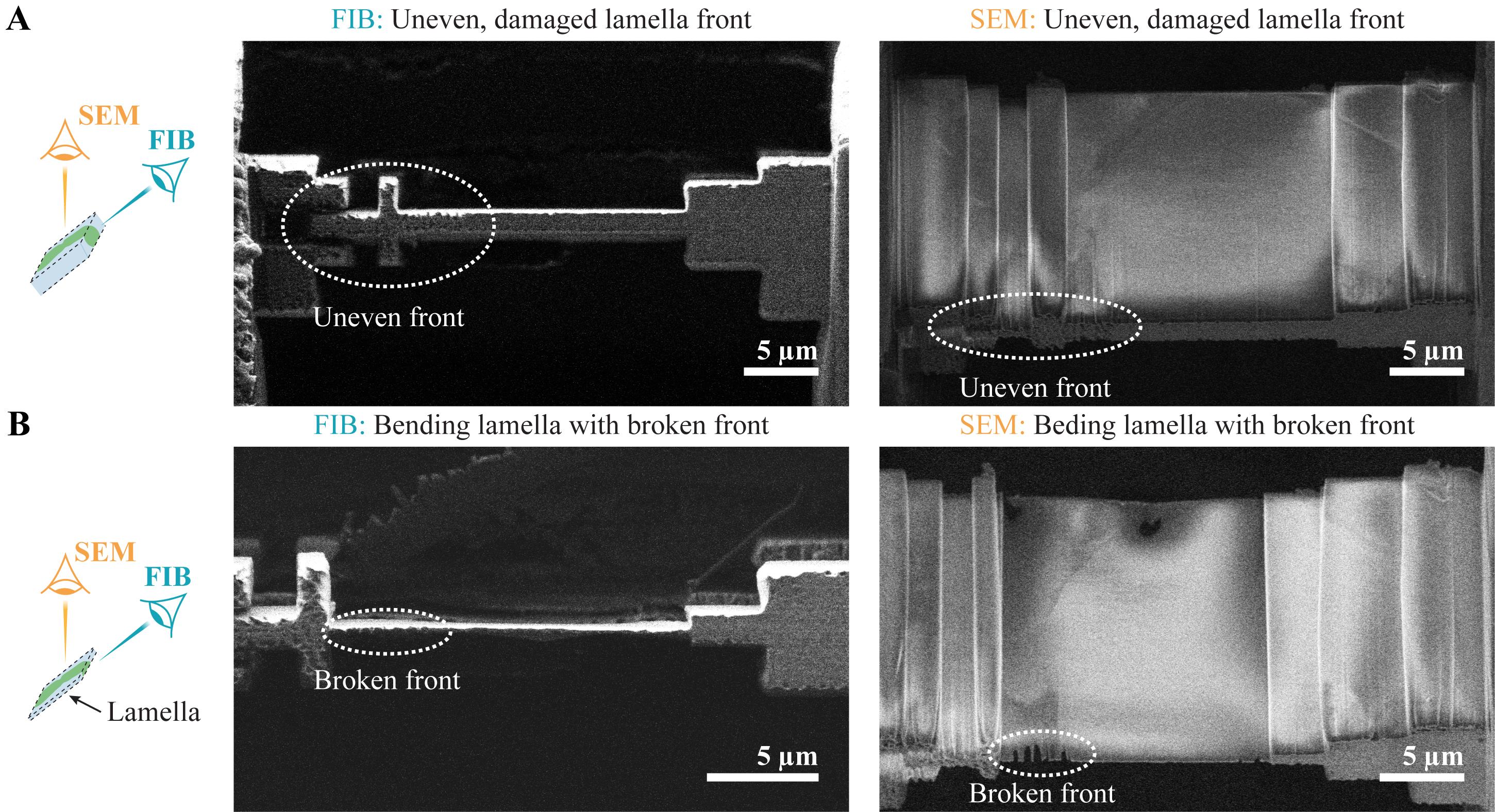
Figure 34. Example of a waffle lamella with a too-thin layer of metal-organic platinum. (A) The waffle lamella before fine milling. The front already appears very uneven. (B) The same lamella after attempting fine milling. The protective layer in the front is broken, and the lamella started bending before it was milled homogeneously thin.
Supplementary information
The following supporting information can be downloaded here:
The supplementary file “FIB_Patterns.zip” contains several subfolders with the FIB milling patterns used:
1. “FIB_Patterns/A_Waffle_Milling” contains the patterns used in Part I, sections D and F.
2. “FIB_Patterns/B_Double_sided_attachment_from_below” contains the patterns used in Part II, sections A and C–E.
3. “FIB_Patterns/C_Double_sided_attachment_from_side” contains the patterns used in Part III, sections A and C.
4. “FIB_Patterns/D_Single_sided_attachment” contains the patterns used in Part IV, sections A and C–E.
Acknowledgments
We thank Manuel Miras and Neda Kazemein Jasemi for their help with the P. patens culture. This work received funding from the European Research Council (ERC SYNERGY Grant agreement “SymPore” no. 951292).
Author contributions
Conceptualization: all authors; Investigation: M.P., M.D., P.X., O.H.S., C.O.J.K., A.B., C.C., S.K.; Writing—Original Draft: M.P., M.D., O.H.S., C.O.J.K., S.K., M.R.; Writing—Review & Editing: all authors; Funding acquisition: W.B.F., R.S., W.X.S., W.B., J.M.P.; Supervision: W.B., J.M.P., W.B.F., R.S., W.X.S.
Competing interests
Jürgen M. Plitzko and Wolfgang Baumeister hold positions on the advisory board of Thermo Fisher Scientific. The other authors declare that no competing interests exist.
References
- Schiøtz, O. H., Kaiser, C. J. O., Klumpe, S., Morado, D. R., Poege, M., Schneider, J., Beck, F., Klebl, D. P., Thompson, C., Plitzko, J. M., et al. (2023). Serial Lift-Out: sampling the molecular anatomy of whole organisms. Nat Methods. 21(9): 1684–1692. https://doi.org/10.1038/s41592-023-02113-5
- Pöge, M., Dickmanns, M., Xu, P., Li, M., Schiøtz, O. H., Kaiser, C. O., Ma, J., Bieber, A., Capitanio, C., Brenner, J., et al. (2025). Making plant tissue accessible for cryo-electron tomography. eLife. 14:RP106455. https://doi.org/10.7554/elife.106455.1
- Lučić, V., Rigort, A. and Baumeister, W. (2013). Cryo-electron tomography: The challenge of doing structural biology in situ. J Cell Biol. 202(3): 407–419. https://doi.org/10.1083/jcb.201304193
- Turk, M. and Baumeister, W. (2020). The promise and the challenges of cryo‐electron tomography. FEBS Lett. 594(20): 3243–3261. https://doi.org/10.1002/1873-3468.13948
- Dubochet, J. (2007). The Physics of Rapid Cooling and Its Implications for Cryoimmobilization of Cells. Methods Cell Biol. 7–21. https://doi.org/10.1016/s0091-679x(06)79001-x
- Dobro, M. J., Melanson, L. A., Jensen, G. J., McDowall, A. W. (2010). Plunge freezing for electron cryomicroscopy. Methods Enzymol. 481: 63–82. https://doi.org/10.1016/S0076-6879(10)81003-1
- Rigort, A., Bäuerlein, F. J. B., Villa, E., Eibauer, M., Laugks, T., Baumeister, W. and Plitzko, J. M. (2012). Focused ion beam micromachining of eukaryotic cells for cryoelectron tomography. Proc Natl Acad Sci USA. 109(12): 4449–4454. https://doi.org/10.1073/pnas.1201333109
- Arnold, J., Mahamid, J., Lucic, V., de Marco, A., Fernandez, J. J., Laugks, T., Mayer, T., Hyman, A. A., Baumeister, W., Plitzko, J. M., et al.(2016). Site-Specific Cryo-focused Ion Beam Sample Preparation Guided by 3D Correlative Microscopy. Biophys J. 110(4): 860–869. https://doi.org/10.1016/j.bpj.2015.10.053
- Yang, J., Vrbovská, V., Franke, T., Sibert, B., Larson, M., Coomes, T., Rigort, A., Mitchels, J. and Wright, E. R. (2023). Precise 3D Localization by Integrated Fluorescence Microscopy (iFLM) for Cryo-FIB-milling and In-situ Cryo-ET. Microsc Microanal. 29: 1055–1057. https://doi.org/10.1093/micmic/ozad067.541
- Koning, R. I., Koster, A. J. and Sharp, T. H. (2018). Advances in cryo-electron tomography for biology and medicine. Ann. Anat. 217: 82–96. https://doi.org/10.1016/j.aanat.2018.02.004
- DUBOCHET, J. (1995). High-pressure freezing for cryoelectron microscopy. Trends Cell Biol. 5(9): 366–368. https://doi.org/10.1016/s0962-8924(00)89071-6
- Moor, H. (1987). Theory and Practice of High Pressure Freezing. In: Steinbrecht, R.A., Zierold, K. (eds) Cryotechniques in Biological Electron Microscopy. Springer, Berlin, Heidelberg. https://doi.org/10.1007/978-3-642-72815-0_8
- Kelley, K., Raczkowski, A. M., Klykov, O., Jaroenlak, P., Bobe, D., Kopylov, M., Eng, E. T., Bhabha, G., Potter, C. S., Carragher, B., et al. (2022). Waffle Method: A general and flexible approach for improving throughput in FIB-milling. Nat Commun. 13(1): e1038/s41467–022–29501–3. https://doi.org/10.1038/s41467-022-29501-3
- Rensing, S. A., Goffinet, B., Meyberg, R., Wu, S. Z. and Bezanilla, M. (2020). The Moss Physcomitrium (Physcomitrella) patens : A Model Organism for Non-Seed Plants. Plant Cell. 32(5): 1361–1376. https://doi.org/10.1105/tpc.19.00828
- Cove, D. J., Perroud, P. F., Charron, A. J., McDaniel, S. F., Khandelwal, A. and Quatrano, R. S. (2009). Culturing the Moss Physcomitrella patens: Figure 1.. Cold Spring Harb Protoc. 2009(2): pdb.prot5136. https://doi.org/10.1101/pdb.prot5136
- Dickmanns, M., Pöge, M., Xu, P., Gombos, S., Barr, Z. K., Miras, M., Plitzko, J. M., Simon, R., Schulze, W. X., Frommer, W. B., et al. (2026). In situ architecture of plasmodesmata in Physcomitrium patens resolved by cryo-electron tomography. Nat Plants. 12(5): 1051–1061. https://doi.org/10.1038/s41477-026-02294-9
文章信息
稿件历史记录
提交日期: Jun 12, 2026
接收日期: Aug 27, 2026
在线发布日期: Oct 8, 2026
出版日期: Oct 20, 2026
版权信息
© 2026 The Author(s); This is an open access article under the CC BY-NC license (https://creativecommons.org/licenses/by-nc/4.0/).
如何引用
Readers should cite both the Bio-protocol article and the original research article where this protocol was used:
- Pöge, M., Dickmanns, M., Xu, P., Schiøtz, O. H., Kaiser, C. O. J., Bieber, A., Capitanio, C., Brenner, J., Riggi, M., Klumpe, S., Schulze, W. X., Simon, R., Frommer, W. B., Plitzko, J. M. and Baumeister, W. (2026). Preparation of Moss Tissue for Cryo-Electron Tomography by High-Pressure Freezing, Focused Ion Beam Milling, and Lift-Out. Bio-protocol 16(20): e5855. DOI: 10.21769/BioProtoc.5855.
- Pöge, M., Dickmanns, M., Xu, P., Li, M., Schiøtz, O. H., Kaiser, C. O., Ma, J., Bieber, A., Capitanio, C., Brenner, J., et al. (2025). Making plant tissue accessible for cryo-electron tomography. eLife. 14:RP106455. https://doi.org/10.7554/elife.106455.1

 Download Citation in RIS Format
分类
植物科学 > 植物细胞生物学 > 细胞成像
细胞生物学 > 细胞成像
您对这篇实验方案有问题吗?
在此处发布您的问题,我们将邀请本文作者来回答。同时,我们会将您的问题发布到Bio-protocol Exchange,以便寻求社区成员的帮助。
 发布问题
发布问题


