


Quantification of Asymmetric Division in Cancer Cells via a Flow Cytometry and Cell Sorting–Based Protocol
基于流式细胞术与细胞分选的癌细胞不对称分裂定量分析方法

(*contributed equally to this work) 发布: 2026年11月05日第16卷第21期 DOI: 10.21769/BioProtoc.5851 浏览次数: 37
评审: Anonymous reviewer(s)
 PDF
 Q&A






Abstract
Asymmetric partitioning of cellular components during division contributes to generating phenotypic heterogeneity and plasticity in genetically identical cells, like bacteria or cancer cells. Traditionally, this partitioning noise has been investigated using live-cell time-lapse confocal microscopy; however, while imaging offers high spatial resolution, it suffers from low statistical throughput and labor-intensive cell tracking. To overcome these limitations, we present a protocol that combines high-throughput flow cytometry and sorting with a theoretical model to precisely quantify partitioning noise during cell division. This method details the experimental setup for measuring cellular components in dividing populations, the data acquisition pipeline, and the implementation of the mathematical framework to extract inheritance parameters. Applicable to both suspension and adherent cells, we have validated our approach against live-cell imaging of adherent colon cancer cells. Hence, this flow cytometry–based approach offers a highly scalable, accessible, and statistically robust alternative to traditional imaging. It is widely applicable across diverse cell lines and biological systems, significantly advancing our capacity to study partitioning-driven phenotypic heterogeneity.
Key features
• A useful and robust method applying flow cytometry to quantify the partitioning noise of cellular components during cancer cell division.
• The theoretical model is able to describe how fluorescence intensities evolve during cell division following cell proliferation.
• Applicable to both suspension and adherent cell lines across multiple cellular components, enabling cross-system comparison of partitioning-driven phenotypic heterogeneity.
Keywords: Asymmetric division (不对称分裂) Partitioning noise (分配噪声)
Flow cytometry (流式细胞术)
Time-lapse microscopy (延时显微成像)
Stochastic modeling (随机建模)
Cell proliferation (细胞增殖)
Cell sorting (细胞分选)
Graphical overview
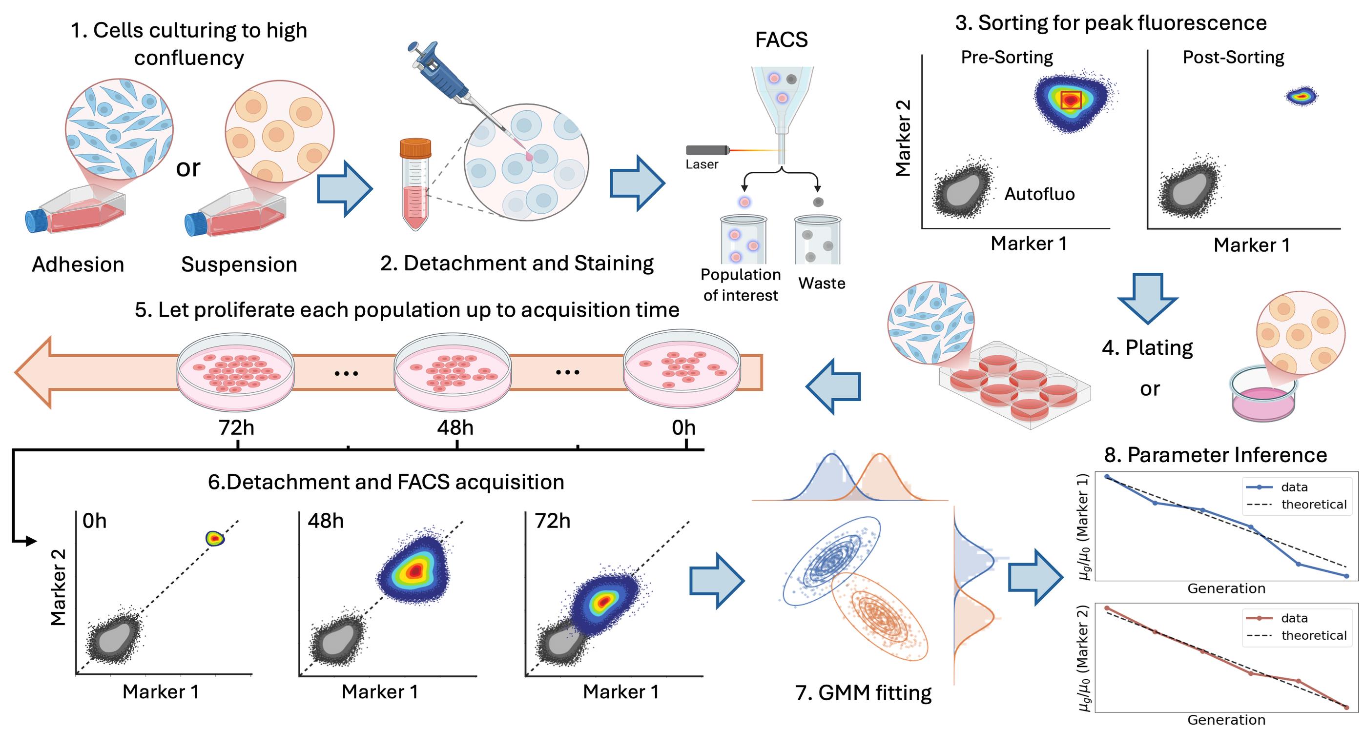
Experimental pipeline and analysis. From top left to bottom right, the figure represents the multiple steps involved in the experimental workflow and the analysis tools required to go from cells in culture to the estimation of the strength of asymmetric component inheritance. 1) Cells are cultured to high confluence; 2) cells are collected (with prior detachment if needed) and stained for specific cellular components using live fluorescent markers (the procedure is described for up to two components); 3) cells are sorted around peak fluorescence; 4) cells are plated in a single- or multi-well format (details in the main text); 5) cells are allowed to proliferate up to the acquisition time; 6) at each acquisition time, a subset of the population is acquired by flow cytometry; 7) raw data are clustered using a Gaussian mixture model (GMM); and finally, 8) an analytical model is fit to infer the strength of fluctuations.
Background
Quantitative analysis of cell proliferation is essential for understanding tissue homeostasis, development, and cancer progression. This is especially true in contexts where cell-to-cell variability emerges during repeated rounds of division. Among the mechanisms contributing to such variability, the unequal inheritance of cellular material at division has attracted increasing attention in the research community [1,2]. Indeed, asymmetric partitioning of fate determinants has been associated with phenotypic diversification of proliferating populations and with cancer cell plasticity, adaptation, and treatment response [3–5]. Experimental quantification of these processes, however, remains challenging. Conventional microscopy-based approaches are often labor-intensive, limited in throughput, and difficult to apply over many generations or across multiple cellular components simultaneously [6,7]. Additionally, for suspension cells, this approach is challenging by itself, requiring the development of ad hoc approaches [8–10], forcing precise control over cell positioning and environmental conditions. Indeed, even small perturbations would disrupt cell positioning, compromising imaging and lineage tracing.
Here, we present a protocol developed across two complementary studies [11,12]. In both, fluorescence-based proliferation assays were combined with statistical modeling to infer the inheritance properties of specific cellular components across successive cell generations. In Peruzzi et al. [11], the protocol was established for suspension cells using multiparametric flow cytometry and multicolor staining. This allowed simultaneous tracking of cytoplasm, membrane lipids, and mitochondria during Jurkat cell proliferation. In the work by Caudo et al. [12], we focused on extending the approach to adherent epithelial cell lines, derived from both cancer and normal human cells, validating the results with extensive time-lapse fluorescence microscopy at the single-cell level.
Our approach demonstrates that a sorting-based strategy coupled to dye-dilution measurements can resolve generation structure over time and, when combined with a statistical framework, can be used to extract quantitative information on the partitioning behavior of different subcellular compartments [11–13]. After each division, the mean fluorescence intensity decreases because the label is distributed between daughter cells, whereas the variance of the fluorescence-intensity distribution reflects the asymmetry of inheritance in this process. Our statistical model predicts the generation-dependent mean and variance of fluorescence distribution from the properties of the partitioning distribution. By sampling large cell populations, flow cytometry enables inference of the statistical consequences of stochastic partitioning by comparing the experimental result with the theoretical prediction. Specifically, while time-lapse fluorescence microscopy enables a detailed characterization of the division process, offering high spatial and temporal resolution and allowing mother-to-daughter lineage tracing, the flow cytometry workflow, combined with a mathematical model of cell division and proliferation [14], provides a robust and high-throughput readout of proliferation history and generation-resolved fluorescence. The details of the mathematical formulation and parameter estimation procedure are explained in the Data analysis section, but we refer to [11,12] for the full derivation.
In this protocol, we describe in detail the procedures for both suspension and adherent cell lines, which required subtle but important modifications to the experimental workflow, as well as the accompanying statistical and computational analysis tools. The protocol thus provides a unified methodological framework derived from these earlier studies and adapted for routine use. Depending on the biological question and the available instrumentation, the workflow can be implemented either with multiparametric staining strategies, enabling the simultaneous tracking of multiple cellular compartments, or with single-parameter measurements, offering a simpler and more accessible implementation.
Finally, we emphasize that the approach presented here can be readily applied to different cell lines and diverse cellular components, providing a powerful and versatile tool for investigating partitioning-driven phenotypic heterogeneity [14–18].
Materials and reagents
Biological materials
1. E 6.1 Jurkat T cells kindly provided by Dr. Nadia Peragine, Department of Cellular Biotechnologies and Hematology, Sapienza University
2. Caco-2 colorectal adenocarcinoma cell line, ATCC (Manassas, VA, USA, HTB-37)
3. HCT116 VIM RFP, colorectal carcinoma cell line, ATCC (Manassas, VA, USA, CCL-247EMT)
4. CCD-18Co, colon fibroblast cell line, ATCC (Manassas, VA, USA, CRL-1459)
Reagents
1. RPMI (Roswell Park Memorial Institute) 1640 medium without L-glutamine with phenol red (SIAL, catalog number: SIAL-RPMI-XA)
2. DMEM (Sigma-Aldrich, catalog number: D6046)
3. DMEM high glucose (Sigma-Aldrich, catalog number: D6546)
4. McCoy’s 5A (Sigma-Aldrich, catalog number: M9309)
5. L-Glutamine 100× (200 mM) (Sigma-Aldrich, catalog number: G7513)
6. Penicillin/Streptomycin 100× (Sigma-Aldrich, catalog number: P4333)
7. Nonessential amino acids (NEAA) (100×) (Gibco, catalog number: 11140-035)
8. Sodium pyruvate (100×) (Gibco, catalog number: 11360-070)
9. Fetal bovine serum (FBS) (Sigma-Aldrich, catalog number: F2442)
10. Trypsin EDTA 0.25% (Sigma-Aldrich, catalog number: T4049)
11. b-Mercaptoethanol (Sigma, catalog number: M3148)
12. Trypan Blue stain 0.4% (Thermo Fisher Scientific, catalog number: T10282)
13. FACSFlow solution 20 L (BD, catalog number: 342003)
14. Clean solution 5 L (BD, catalog number: 340345)
15. BDTM detergent solution concentrate FAC (BD, catalog number: 660585)
16. BD FACSTM Cytometer Setup & Tracking Beads K (CS&T) (BD, catalog number: 642412)
17. BD FACSTM Accudrop Fluorescent Beads (BD, catalog number: 345249)
18. Countess cell counting chamber slides (Thermo Fisher Scientific, catalog number: C10283)
19. Dulbecco’s phosphate buffer saline (PBS) solution w/o Ca++ and Mg++ (Euroclone, catalog number: ECB4004L)
20. Dimethyl sulfoxide (DMSO) (Sigma-Aldrich, catalog number: D5879)
21. Ethanol absolute (Sigma-Aldrich, catalog number: 32221-2.5L-M)
22. Bovine serum albumin (BSA) (Sigma, catalog number: A07030)
23. Ethylenediaminetetraacetic acid disodium salt solution (EDTA) (Sigma-Aldrich, catalog number: E7889)
24. Fixable Viability Stain 780 (FVS780) (BD Horizon, catalog number: 565388)
25. CellTraceTM Violet Cell Proliferation kit (Thermo Fisher Scientific, catalog number: C34557)
26. CellTraceTM Yellow Cell Proliferation kit (Thermo Fisher Scientific, catalog number: C34567)
27. CellTraceTM Far Red Cell Proliferation kit (Thermo Fisher Scientific, catalog number: C34564)
28. MitoTracker Deep Red FM (Thermo Fisher Scientific, catalog number: M22426)
29. MitoTrackerTM Green FM (Thermo Fisher Scientific, catalog number: M7514)
30. PKH26 Red Fluorescent Cell Linker Mini kit (Sigma-Aldrich, catalog number: MINI26-1KT)
Solutions
1. Sorting buffer (see Recipes)
2. EtOH 70% (see Recipes)
3. RPMI 1640 growth medium (see Recipes)
4. DMEM growth medium 20% (see Recipes)
5. DMEM growth medium 10% (see Recipes)
6. McCoy’s 5A growth medium (see Recipes)
7. Fluorescent dye (see Recipes)
Recipes
1. Sorting buffer
| Reagent | Final concentration | Quantity or volume |
|---|---|---|
| PBS | n/a | q.s. to 100 mL |
| FBS | 2% | 2 mL |
| EDTA | 0.5 mM | 100 μL |
Store at 4 °C.
2. EtOH 70%
| Reagent | Final concentration | Quantity or volume |
|---|---|---|
| diH2O | 30% | 30 mL |
| EtOH | 70% | 70 mL |
3. RPMI 1640 growth medium
| Reagent | Final concentration | Quantity or volume |
|---|---|---|
| RPMI 1640 | 88% | 88 mL |
| FBS | 10% | 10 mL |
| Penicillin/Streptomycin | 1% | 1 mL |
| Glutamine | 1% | 1 mL |
Used for E6.1 Jurkat cell maintenance.
4. DMEM growth medium 20%
| Reagent | Final concentration | Quantity or volume |
|---|---|---|
| DMEM (D6046) | 76% | 76 mL |
| FBS | 20% | 20 mL |
| Penicillin/Streptomycin | 1% | 1 mL |
| Glutamine | 1% | 1 mL |
| NEAA | 1% | 1 mL |
| Sodium pyruvate | 1% | 1 mL |
Used for Caco-2 (ATCC HTB-37) cell maintenance.
5. DMEM growth medium 10%
| Reagent | Final concentration | Quantity or volume |
|---|---|---|
| DMEM (D6046) | 86% | 86 mL |
| FBS | 10% | 10 mL |
| Penicillin/Streptomycin | 1% | 1 mL |
| Glutamine | 1% | 1 mL |
| NEAA | 1% | 1 mL |
| Sodium pyruvate | 1% | 1 mL |
Used for CCD18Co (ATCC CRL-1459) cell maintenance.
6. McCoy’s 5A growth medium
| Reagent | Final concentration | Quantity or volume |
|---|---|---|
| McCoy’s 5A (M9309) | 88% | 88 mL |
| FBS | 10% | 10 mL |
| Penicillin/Streptomycin | 1% | 1 mL |
| Glutamine | 1% | 1 mL |
Used for HCT-116 VIM RFP (ATCC CCL-247EMT) cell maintenance.
7. Fluorescent dye
| Dye | Excitation/emission peaks | Quantity or volume |
|---|---|---|
| CellTraceTM Violet | 392/456 nm | 1/1,000 from 5 mM in DMSO |
| MitoTrackerTM Green | 490/516 nm | 1/1,000 from 20 µM in DMSO |
| Fixable Viability Stain 780 | 759/780 nm | 1/1,000 from 0.6 mM in DMSO |
| PKH26 | 551/567 nm | 4 µL in 1 mL of diluent C; final concentration: 2 µM |
Laboratory supplies
1. 15 mL conical centrifuge tubes, polypropylene, sterile (Falcon, Corning, catalog number: 352096)
2. 50 mL conical centrifuge tubes (Falcon, Corning, catalog number: 352070)
3. Filter system 250–500 mL (Corning, catalog numbers: 431096 and 431097)
4. Round-bottom polystyrene tubes 5 mL (BD, catalog number: 352054)
5. Round-bottom polypropylene tubes 5 mL (BD, catalog number: 352063)
6. Eppendorf safe-lock tubes, 1.5 mL (Eppendorf, catalog number: 0030123328)
7. P10–P1000 tips, sterile (Sial, catalog numbers: SIAL-UTF10-10, SIAL-UT200-10, and SIAL-UT1000-R)
8. Serological pipettes, 2–25 mL, sterile (Costar, Corning, catalog numbers: 4486, 4487, 4488, and 4489)
9. Cell culture wells: 6–24 well, 96 wells (Costar, Corning, catalog numbers: 3516, 3524, and 3799)
10. Cell culture plates: T25–75 (Corning catalog numbers: 430639 and 430641U)
11. Syringe BD Plastipak 5 mL, Luer Lock, sterile (BD, catalog number: 309649)
12. FilconTM syringe-type, sterile, 50 μm (BD, catalog number: 340602)
13. Cell imaging μ-dish 35 mm and μ-slide 4-well ibiTreat (IBIDI, catalog number: 80426)
Equipment
1. Class II microbiological safety cabinet (Thermo Scientific, model: MSC 1.2)
2. Water bath (Memmert, Germany; model: WNB10)
3. Freezer (-20 °C) (Liebherr Scientific)
4. Refrigerator (2–8 °C) (Liebherr Scientific)
5. Liquid nitrogen tank
6. Serological pipettes and micropipettes (standard sizes, sterile)
7. Incubator, 150 L (Thermo Scientific, model: HERAcell 150i CO2)
8. Microscope capable of 10×, 20×, and 40× magnification in brightfield
9. Hemocytometer
10. Countess 3 Automated Cell Counter (Thermo Fisher Scientific)
11. Centrifuge (Thermo Scientific, model: SL-16R)
12. Inverted microscope (Zeiss, model: PrimoVert)
13. Inverted microscope (Zeiss, model: AX10 Vert.A1 FL-LED)
14. Olympus FluoView FV1200 confocal laser scanning microscope (built on IX83 inverted frame) (Olympus Corporation, model: FV1200-IX83) equipped with a 20× air objective (Olympus, Shinjuku, Japan) and an on-stage incubator
15. Freezing container Nalgene Mr. Frosty (Sigma-Aldrich, catalog number: C1562)
16. BD FACSARIA III Cell Sorter 648282 (Becton Dickinson)
17. BD LSRFortessa Cell Analyzer 647797 (Becton Dickinson)
Software and datasets
1. FACSDiva software, version 6.1.3 (Beckton Dickinson), for FACS acquisition
2. FlowJo software, version 10.10.0 (Beckton Dickinson), for FACS data analysis
3. Fiji software, version 1.0, for confocal microscopy image segmentation
4. Zen Microscopy Software (ZEISS), for microscopy acquisition
5. In-house developed Python program
Procedure
Before initiating procedures, ensure a sterile working environment by thoroughly disinfecting the biosafety cabinet interior (work surface and walls) and all necessary materials with diH2O and 70% ethanol, then exposing the cabinet to UV light for 60 min. All subsequent steps must be performed under strict aseptic conditions within the prepared workspace, after allowing the surface to air-dry completely.
We present the procedures in parallel for the adherent cell lines (CaCO-2, CCD18Co, HCT-116 VIM RFP) and the suspension cells (Jurkat T cells). For the sake of readability, we do not repeat the procedures for every cell line. Hence, when reading complete media (cMedia), the reader must refer to the correct one for each cell line, as indicated in Table 1. All cell lines used have been routinely tested for mycoplasma.
Table 1. Association between complete Medium (cMedia) and cell lines
| Caco-2 | CCD18Co | HCT-116 VIM RFP | Jurkat |
| cDMEM 20% | cDMEM 10% | cMcCoy’s 5A 10% | cRPMI 10% |
A. Thawing
1. Prepare a 15 mL Falcon tube with 9 mL of cMedia at 4 °C.
2. Prepare a T75 (or T25) flask with 18 mL (3 mL) of cMedia and store it at 37 °C.
3. Remove the vial containing the cells from the liquid nitrogen storage.
4. Place it in a prewarmed water bath at 37 °C for approximately 2 min, until the liquid starts melting.
5. With a 1,000 μL Gilson pipette, add to the vial 1 mL of cMedia at 4 °C. Mix rapidly to complete thawing.
6. Transfer the thawed cells with a 1,000 μL Gilson pipette into the 15 mL Falcon tube with the remaining cMedia.
7. Centrifuge at 368× g or 1400 rpm for 7 min.
8. Resuspend cells in 2 mL of cMedia.
9. Plate them in the prewarmed T75 (or T25) flask.
Critical:
1. The flask’s size depends on the number of cells thawed. We suggest the T75 for around 106 cells and above.
2. The media in the 15 mL Falcon has to be cold to avoid thermal shock.
3. The media in the flask has to be put at 37 °C to favor faster settlement to optimal proliferation after thawing.
B. Cell culture
The different cell lines are used as different cell models for proliferation studies. Jurkat cells are representative of suspension cells, while Caco-2, CCD18Co, and HCT-116 VIM RFP are representative of adherent cells. Each line is cultured in appropriate cMedia (see Recipes and Table 1), maintained in an incubator humidified with 95% air and 5% CO2 at 37 °C. To achieve cell recovery post-thawing, cells are passaged once in a T75 flask prior to amplification for the experiment.
1. Suspension cell culture
a. Jurkat cells are cultured in a T75 flask in a final volume of 20 mL. To passage suspension cells, gently disaggregate the cell clusters and chains of actively growing cells with a 5 mL pipette, collect the cells in 15 mL conical polypropylene and sterile centrifuge tubes, and spin at 368× g or 1,400 rpm for 7 min.
b. Resuspend harvested cells in PBS, count, and divide into additional T75 flasks for amplification according to experimental needs, considering their doubling time of 18–20 h. Generally, prior to the experiment, by plating 6–8 T75 flasks containing 2 × 10⁶ in 20 mL of growth medium, the harvest for the experiment after three days of culture yields a total of 60–80 × 106 cells.
2. Adherent cell culture
a. To passage adherent cells, remove the medium from the T75 flask and wash it with 5 mL of PBS. Add 2 mL of Trypsin EDTA 0.25% for 2 min at 37 °C. After checking the detachment state with an inverted microscope, mechanically agitate the flask to favor detachment. Neutralize trypsin with 4 mL of cMedia in a 5 mL pipette and quickly but vigorously mix. Transfer the volume into a 15 mL Falcon tube. Wash the flask with 4 mL of cMedia. Transfer the volume to the same 15 mL Falcon tube and dilute with 4 mL of PBS. Centrifuge at 368× g or 1,400 rpm for 7 min.
b. Resuspend the pellet in 10 mL of PBS and centrifuge again at 368× g or 1,400 rpm for 7 min.
c. Resuspend in 2 mL of cMedia and plate in a pre-wet T75 flask with 18 mL of room-temperature cMedia.
Critical:
1. Handle cells and use all related reagents in sterile conditions under the laminar flow hood. Mixing vigorously after trypsin addition with a 5 mL pipette is a fundamental step to avoid the presence of cell aggregates.
2. For adherent cells, efficient detachment is essential to obtain a homogeneous single-cell suspension. The optimal detachment procedure may vary according to the cell line and the level of culture confluence. Therefore, detachment should be visually verified before applying mechanical stress, and the trypsin incubation time should be adjusted as necessary. Under the experimental conditions described in this protocol, the indicated trypsin incubation time was sufficient to achieve effective cell detachment.
3. Careful pipetting after trypsin neutralization is important to disperse residual cell aggregates. Using a smaller-volume pipette, such as a 2 mL serological pipette, can increase shear stress and improve dissociation.
C. Cell fluorescent dye labeling to track cell proliferation
To track cell proliferation by dye dilution, establishing the daughter progeny of a completed cell cycle, cells were stained with CellTraceTM Violet and MitoTrackerTM Green FM or PKH26, typically used to monitor multiple cell generations. The use of different markers for cytoplasm, mitochondria, or cell membrane allowed for a multivariable proliferation analysis.
1. Prepare a cell suspension of the sample.
2. Upon extensive washing in PBS (centrifuge at 368× g or 1,400 rpm for 7 min), count viable cells with a cell counter using the dye exclusion test of Trypan Blue solution, an impermeable dye not taken up by viable cells.
3. Prepare 1 mL of cell suspension in a 15 mL conical, polypropylene, sterile tube, including 20 × 106 cells in PBS (2 × 10⁷ cells/mL). Label as a stained sample.
4. Prepare an additional FACS tube containing 0.5 × 10⁶ cells/100 μL of PBS and keep at 4 °C. This represents the unstained sample.
5. As the first staining to discriminate viable cells, Fixable Viability Stain 780 (FVS780) is used. Incubate cells resuspended in protein-free PBS at room temperature for 10 min, protected from light, with FVS780 at a final concentration of 1/1,000 from stock (stocks prepared as indicated in the reagent datasheet).
6. Upon staining, ensure to wash twice the cell suspension with PBS (centrifuge at 368× g or 1,400 rpm for 7 min) containing a low amount of FBS (2%) to quench the reactivity of the free dye.
7. Decant the supernatant, gently mix to disrupt the cell pellet, and resuspend the cells in PBS for the subsequent staining of cytoplasm and mitochondria dyes, or in diluent C for lipophilic dyes for membrane staining
8. If membrane staining is required, follow the steps below; otherwise, proceed directly to step C9:
a. Add an equal volume of the cell suspension to the 2× dye solution. Prepare the 2× dye solution immediately before use by adding 4 μL of PKH26 to 1 mL of diluent C, resulting in a final PKH26 concentration of 4 μM in the 2× dye solution.
b. Incubate the cell suspension with the 2× dye solution under gentle agitation for 2 min at room temperature.
c. Immediately quench the staining by adding an equal volume of FBS and top up the tube with 10 mL of cMedia.
d. Wash the cells with PBS by centrifugation at 368 × g (1,400 rpm) for 7 min.
e. Resuspend the cells in PBS for subsequent cytoplasmic staining.
9. Add CellTraceTM Violet dye according to the manufacturer’s instructions (1/1,000 dilution from the mother stock 5 mM in DMSO) for 25 min at room temperature protected from light, mixing every 10 min to ensure homogeneous cell labeling in the stained sample.
10. Afterward, add 5× complete media to the cell suspension for an additional 5-min incubation before washing in PBS (centrifuge at 368× g or 1,400 rpm for 7 min).
11. If mitochondrial staining is intended, follow the steps below; otherwise, skip directly to step C12:
a. Decant the supernatant, gently mix to disrupt the cell pellet, and resuspend the cells in 1 mL of PBS.
b. Add MitoTrackerTM Green FM, a green fluorescent mitochondria stain, according to the manufacturer’s instructions (1/1,000 dilution from the mother stock 20 μM in DMSO) for 30 min in a water bath at 37 °C, mixing every 10 min to ensure homogeneous cell labeling in the stained sample.
c. Wash stained cells in PBS (centrifuge at 368× g or 1,400 rpm for 7 min), filling the 15-mL tube upon each staining. Add 6 mL of PBS and centrifuge the cells at 368× g or 1,400 rpm for 7 min.
d. Discard the supernatant, resuspend the pelleted cells in 12 mL of PBS, and centrifuge the cells again at 368× g or 1,400 rpm for 7 min. This is the final washing.
12. Dislodge the cell pellet in 0.5 mL of sorting buffer in a sterile, round-bottom polypropylene 5 mL tube.
13. Pass the cell suspension through a sterile syringe-mounted filter (50 µm) immediately before sample loading to remove residual cell aggregates, prevent clogging of the sorter fluidics, and improve single-cell dissociation.
Critical:
1. To avoid fluorescence quenching, protect the stained sample from direct light exposure, covering the tube with aluminum foil.
2. Make sure to perform all staining procedures in sterile conditions under the laminar flow hood, since isolated cells will be cultured.
3. All the dyes are preserved at -20 °C in DMSO aliquots, which are prepared for single usage in order to avoid excessive exposure to air and moisture, which would impair reproducibility and correct effective staining.
4. A relatively high number of stained cells (2 × 10⁷ cells/mL) is recommended before sorting for adherent cell lines and kinetic experiments requiring the collection of multiple time points. The sorting strategy generally uses a narrow gate centered on the upper fluorescence range of the two staining parameters; consequently, only a fraction of the stained population is recovered. Starting from a larger cell number helps ensure that sufficient highly labeled cells are collected for subsequent plating and longitudinal analysis. A high starting cell number also compensates for potential variability in labeling efficiency. If staining is not homogeneous, fewer cells may fall within the selected high-fluorescence gate. In addition, adherent cells require enzymatic detachment and mechanical dissociation before sorting and may partially re-aggregate during sample handling. Retaining an additional stained cell fraction from the same preparation provides a backup sample in case of aggregation, reduced sorting efficiency, or other technical issues during the sorting procedure.
D. Cell sorting
The BD FACSAria III (Becton Dickinson) is equipped with four lasers: near UV 375 nm, 488 nm, 561 nm, and 633 nm. It runs the FACSDiva software (BD Biosciences, version 6.1.3).
1. Start up the BD FACSAria III cell sorter.
a. Before starting, check the fluid tanks. Refill the sheath fluid tank with FACSFlow solution and discard the waste container. Also, check the EtOH tank. Ensure that it contains enough 70% EtOH for the shutdown procedure.
b. Start up the workstation and, after 1 min, turn on the cell sorter main power and then run the FACSDiva software, version 6.1.3.
c. Perform Fluidic Startup and start the instrument stream.
d. Ensure cytometer performance is checked by running the Cytometer Setup and Tracking Beads following the application guide.
2. Select the experiment and setup for sorting:
a. Select a new experiment and open a specimen and a tube.
b. In the Inspector-Cytometer settings, insert the parameters for each channel of the experiment, including morphological ones, side and forward scatter, FSC-A and SSC-A, including -H and -W for doublets exclusion.
c. Create dot plots and histograms, including gates to identify the cells to collect. Remember to record 50,000 events per sample to sort.
d. Set up for sorting by performing first the Test Sort, adjusting the voltage to center the collection tube, and then running the Accudrop Fluorescent Beads to determine the drop delay.
e. Create a new Sort Layout where you select the collection device and set the sort precision mode to Purity (two tubes).
3. Sorting procedure:
a. Acquire the unstained sample to set the background fluorescence for each channel.
b. Insert the proper collection devices in the sort collector chamber and load the stained sample for sorting.
c. Cells are gated on single cells by doublet exclusion with morphology parameters, area versus width (A versus W). For each fluorochrome, in the cell population, a sorting gate is set around the max peak of fluorescence of the dye distribution (see Figure 1). This way, collected cells are enriched for the highest fluorescence intensity for the markers used. Once the sorting gate is established, start the sorting.
d. Following isolation, an aliquot of the sorted cells is analyzed at the cell sorter to determine the purity and population width, resulting in an enrichment of >97% for each sample. As shown in Figure 1, the post-sorting acquisition is centered around the sorting gate, although it still presents some variability.
e. Perform the Fluidics Shutdown procedure according to the manufacturer’s instructions, including multiple washing cycles with Clean Solution and BD™ Detergent Solution. Turn off the system upon completion.
Critical: Sorting the population around the fluorescence peak is a critical feature of the protocol. It plays a dual role; it indirectly induces cell synchronization and enables a clearer reconstruction of the coexisting generations. A better description of its role can be found in the General notes.
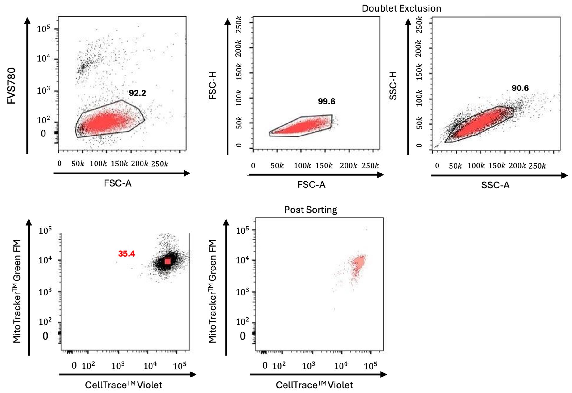
Figure 1. Gate strategy for isolation of Mito/CTV double-positive Jurkat cells. Representative dot plots of Jurkat cells showing the gating strategy for isolation of CTV/Mito highly positive cells. Live cells were first gated based on forward scatter area parameter (FSC-A), and the negativity for the Fixable Viability Stain 780 (FVS780) indicating high viable cells, 92.2%. After that, cells were selected for doublet exclusion (Heights, H versus Area, A for both FSC and side scatter; upper panels) and finally collected based on Mito and CTV highest expression level (left lower panels). Double-positive cell sorting efficiency is shown in the right lower panel. To show the sorted cells (light red), a back-gating strategy is used in all plots to identify the cell population and to confirm the gating strategy.
E. Time course kinetics to assess dye dilution using flow cytometry
The LSRFortessa flow cytometer used to monitor cell proliferation is equipped with five different lasers with the capacity of detecting simultaneously up to 18 distinct colors. The lasers are 355, 405, 488, 561, and 639 nm. The 561 nm laser, named Yellow/Green, allows better resolution of all PE and PE-like fluorophores being excited by a laser closer to the max emission peak of fluorescence.
1. In order to set the time zero of the kinetic, prior to culturing, analyze a tiny aliquot (approximately 30 μL) of the sorted cells immediately after sorting at the flow cytometer. This procedure is required to establish the starting point of the experiment at which the fluorescence levels of the selected markers have the highest intensities.
2. Upon sorting, seed the cells into different plate types and follow over time to monitor multiple cell divisions up to 72 h. To follow the decrease in fluorescence intensities for each used marker, establish a time course kinetics every 18, 24, 36, 48, 60, and 72 h. As depicted in the graphical abstract, according to the cell type used, the plating condition for the time course experiment changes. An example acquisition that follows the dilution of a single marker is shown in Figure 2, where each curve is the fluorescence intensity distribution of the cell population at the acquisition time point. The grey one is the autofluorescence, while the others are the different time points at increasing times from the bottom to the top.
3. For suspension cells, the kinetics are facilitated:
a. Seed sorted cells into a single well of a 6-well plate.
b. Each time point, mix cells by pipetting with a 1,000 μL Gilson pipette.
c. Acquire an aliquot of 350 μL of the growing cell colony at the LSRFortessa.
d. After acquisition, add 350 μL of cMedia to the culture to maintain initial growing conditions.
4. For adherent cells:
a. Seed sorted cells in 12-well plates at a cell density of 30–70 ×103 cells/well, according to the experiment, and keep in culture for up to 84 h. In this case, each well represents a time point of the experimental kinetics acquired every 24, 36, 48, 60, 72, and 84 h, since adherent cells cannot be detached in part from a growing culture. Each time, a whole population is acquired, without subsequent replating.
b. Gently wash the well with 2 mL of PBS.
c. Add 1 mL of Trypsin EDTA 0.25% for 2 min at 37 °C.
d. After checking the state of detachment under the inverted microscope, inactivate trypsin with 1 mL of cMedia.
e. Collect cells in a 15 mL Falcon tube after thorough mixing and pipetting with a 1,000 μL Gilson pipette to ensure full detachment.
f. Wash the well with 3 mL of PBS and then add to the 15 mL Falcon tube.
g. Upon addition of 6 mL of PBS, centrifuge the cells at 368× g or 14,00 rpm for 7 min.
h. Resuspend cells in 300 μL of sorting buffer.
i. Transfer into a FACS tube ready for acquisition.
5. Starting the cytometer:
a. Turn on the flow cytometer and allow 30 min for the optical system to stabilize the temperature prior to starting.
b. Check the tanks prior to starting, ensuring to fill the sheath tank and empty the waste one, and, if present, remove air bubbles trapped in the sheath filter.
c. Prime the fluidics pressing the specific control button to force the fluid out of the flow cell into the waste container; repeat this step during the warming up of the system up to 3–5 times.
d. Leave the cytometer in standby mode until it is ready to run the samples.
6. Acquire the samples:
a. Turn on the computer and launch the FACSDiva software.
b. Select a new experiment and rename it with data and specifics, i.e., Jurkat proliferation kinetic CTV and MFR.
c. Load your samples; the unstained sample is used to set the background fluorescence for each parameter used as described above. Load the stained sample.
d. Create dot plots and histograms to identify the cell population (events) to collect.
e. Select all parameters/channels required for the acquisition of the experiment, and acquire your stained sample.
Critical: Thorough pipetting when detaching adherent cells for the time acquisition is fundamental. Due to the plating support, which does not allow mechanical detachment, pipetting with a 1,000 μL Gilson allows avoiding aggregates and ensuring the full collection of the sample.
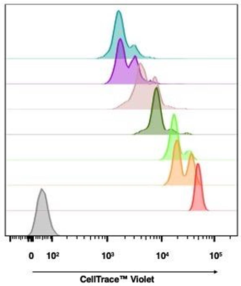
Figure 2. Time course kinetics showing CTV (CellTrace Violet) fluorescence intensity decrease in proliferating Jurkat cells. Representative histogram plot of Jurkat cells showing the fluorescence intensity decrease of CTV during a kinetic experiment. Starting at time 0 (light red), with time increasing from 18, 24, 36, 48, 60, to 72 h (light blue), the proliferating cells show a decrease in fluorescence intensity.
Data analysis
A. Gaussian mixture model
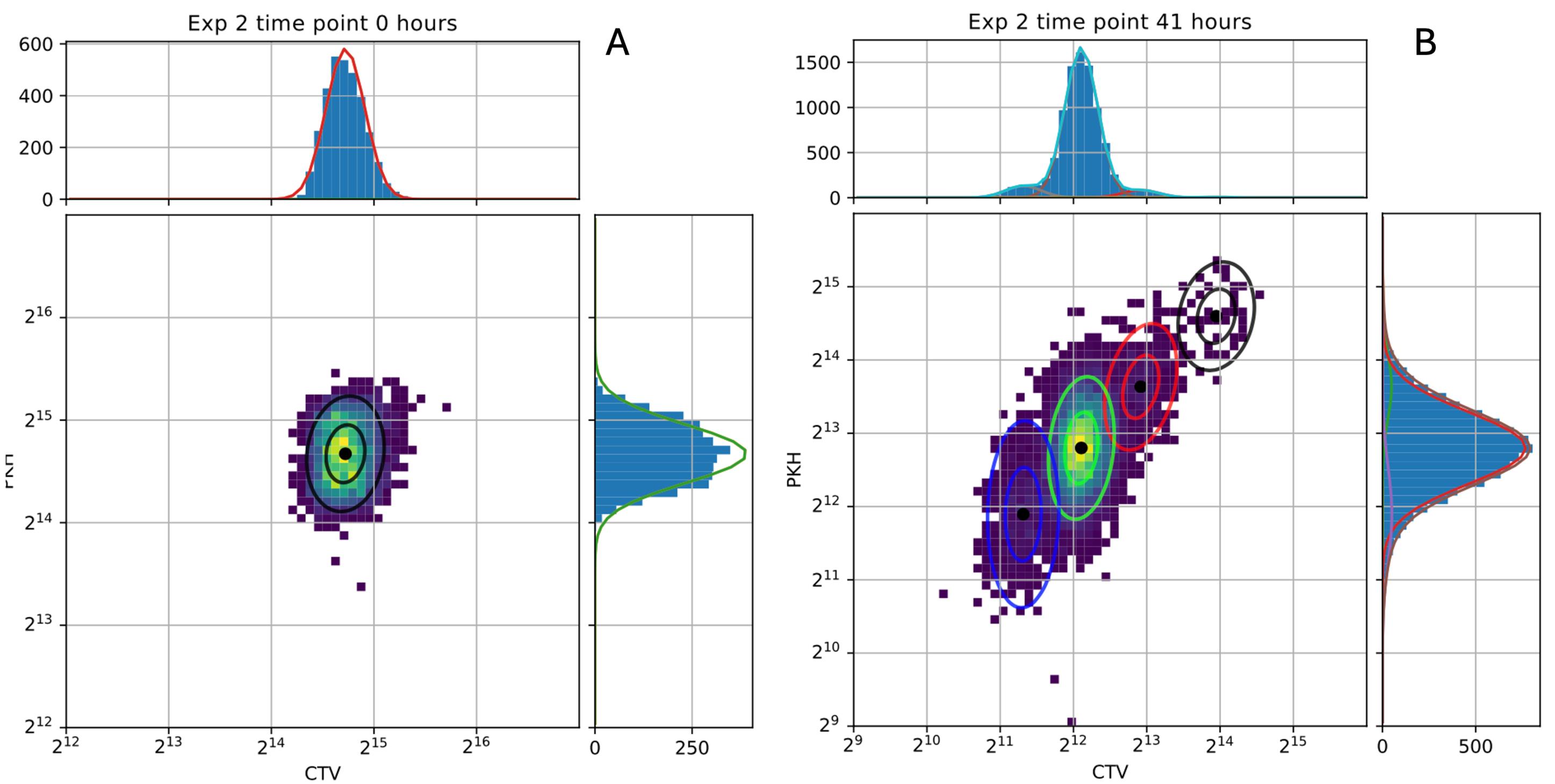
Figure 3. Gaussian mixture model analysis. Two-dimensional density distributions at the 0 and 41-h time points, with marginal one-dimensional distributions for CTV (CellTrace Violet) and PKH26 shown along each axis. The fitted Gaussian mixture models accurately reproduce the observed peaks on a logarithmic scale. Goodness of fit was assessed via the residual sum of squares computed on the normalized distributions, yielding Σ = 6.4 × 10⁻⁴ at 0 h and Σ = 1.12 × 10⁻⁴ at 41 h (where a value of 1 would indicate completely non-overlapping distributions).
The expectation–maximization (EM) algorithm was employed to identify clusters within Gaussian mixture models [19]. This procedure alternates between two steps: the expectation (E) step and the maximization (M) step. In the E step, the current parameter estimates πg, μg, σg, and g are used to compute the posterior probability γg = p(f) for each observation f, representing the probability that a cell with fluorescence intensity belongs to generation g.
In the M step, updated estimates of πg, μg, and σg are obtained by maximizing the log-likelihood of the observed data, with closed-form updates expressed as functions of γg. Under standard regularity conditions, iterating between the E and M steps is guaranteed to converge to a locally optimal parameter set, yielding posterior weights that quantify the degree of cluster membership for each observation. This framework was applied to detect fluorescence intensity peaks corresponding to distinct cell generations, from which the parameters πg, (f > g), and Var[fg] were subsequently estimated.
An example outcome of this fitting procedure is presented in Figure 3. The cell population is tracked during proliferation, and fluorescence intensities are measured at two time points. The different generations are identified by different colors, and the goodness of fit is assessed from the marginal distributions along both axes.
B. Theoretical prediction for the partition process
To describe the evolution of a fluorescently tagged cellular component across a proliferating population, we developed a stochastic model that allows the derivation of the parameters of the partitioning process from experimentally measured means and variances of the fluorescence intensity peaks.
The theoretical framework is grounded in a minimal set of assumptions: (i) cells follow a common division rule, which means that when a cell divides into two daughter cells, each cell inherits a fraction f (or 1-f) of the mother cell component randomly extracted from a distribution Π(f). No specific assumptions are required on the shape or properties of Π(f). (ii) Production and degradation of the tagged component are neglected, reducing the dynamics to a progressive dilution driven solely by partitioning noise, an assumption justified by the use of non-endogenous live fluorescent dyes.
Under these conditions, the full fluorescence distribution of daughter cells can be derived analytically from that of the mother, and by iterating this computation, one can trace the distribution dynamics across any number of generations.
Given an initial distribution of components P(m0), with mean μ0 and variance , it is possible to write the expected value for the mean and variance of the distribution of components at generation g:
The mean does not carry information on the partitioning process itself but describes the progressive dilution of the fluorescent signal across generations. The variance, by contrast, depends directly on the second moment of the partition distribution Π(f). By fitting these expressions to the generation-wise means and variances extracted from flow cytometry data via the Gaussian mixture model, one can obtain a quantitative estimate of the variance of the partitioning process. An explanatory representation of the approach is presented in Figure 4. In a single division event, the post-division fluorescence intensity distribution is the convolution between the initial one and the partitioning distribution probability, which measures how probable it is to inherit a certain fraction of the mother’s component. The single distribution then splits into two subpopulations, one centered in μ0f and one in μ00(1-f) for symmetricity. We can therefore simply compute what the resulting mean and variance of this convolution are. By iterating this concept, the equations for the single event can be extended to a random number of generations g, which will present a higher number of subpopulations corresponding to all the possible combinations of g products between f and 1-f. In Figure 4, we report only the case for g = 2 due to space and feasibility.
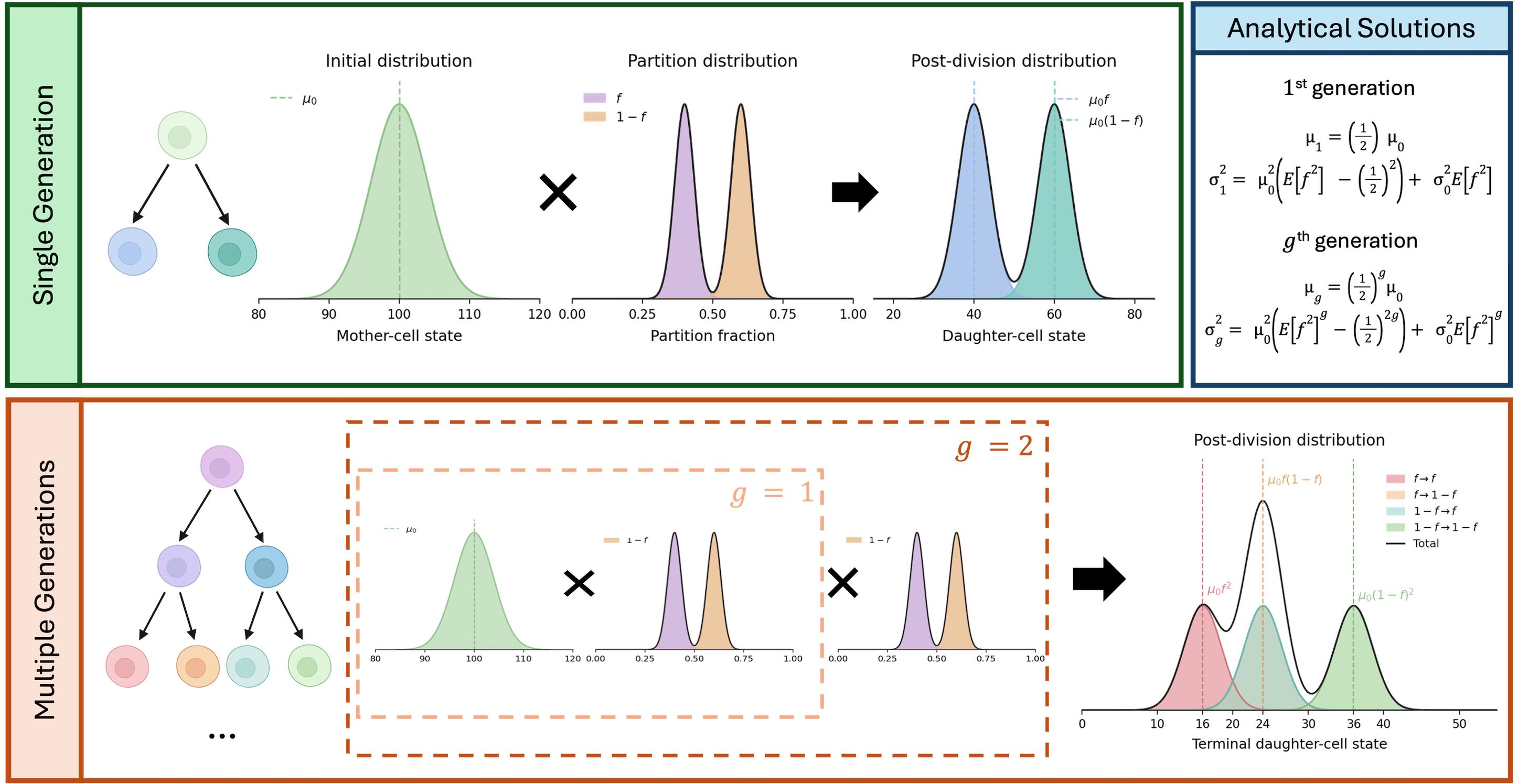
Figure 4. Analytical formula for the g-th generation. A single cell-division event corresponds to combining the initial fluorescence-intensity distribution of a cell population with the partition distribution. This process produces a bimodal daughter-cell distribution, with peaks centered at μ0f and μ0(1-f), where μ0 is the mean initial fluorescence intensity. When this process is repeated over multiple generations—two in our example—the resulting distribution comprises several subpopulations, each corresponding to a possible sequence of inheritance fractions across successive divisions. The upper-right box reports the analytical expressions for the mean and variance of the daughter-cell fluorescence-intensity distribution after one generation, together with their general form for the g-th generation.
Validation of protocol
To validate the results obtained with flow cytometry, time-lapse fluorescence microscopy experiments were performed independently of the flow cytometry time courses. This validation was restricted to adherent cell lines, as lineage tracing in suspension cells would require microfluidic immobilization devices to keep cells within the field of view. Alternative approaches, such as embedding cells in a gel matrix, would excessively alter proliferative conditions and compromise the validity of the measurements. Figure 5 shows an overview of the steps used for microscopy experiments.
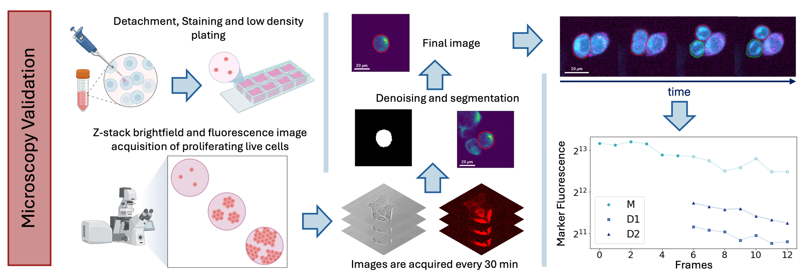
Figure 5. Validation experiment. Adherent cells were detached, stained, and plated at low density in imaging chambers and followed by confocal time-lapse microscopy for three days under controlled culture conditions. Brightfield and fluorescence z-stacks were acquired every 30 min, and the resulting images were analyzed to quantify fluorescence inheritance in daughter cells after division, providing an independent validation of the flow cytometry–based measurements.
1. Cells were amplified under standard growth conditions until reaching ~80% confluence in a T75 flask. They were then detached and collected following the same procedure described for the flow cytometry time course and sorting experiments (see Procedure). Cells were resuspended in 500 μL and counted using Trypan Blue exclusion at 1/10 and 1/100 dilutions.
2. Staining was performed with MitoTracker Deep Red FM (1/1,000 dilution from a 2 mM stock in DMSO) and CellTrace Yellow (1/500 dilution from a 5 mM stock in DMSO) for 25 min at room temperature, protected from light, with gentle mixing every 10 min to ensure homogeneous labeling. Following staining, 5× volume of complete medium was added to the cell suspension for an additional 5-min incubation, after which cells were washed in PBS and resuspended in 1 mL of complete medium (cMedia).
3. An μ-slide 4-well ibiTreat imaging chamber was pre-wetted with 300 μL of cMedia per well. Cells were plated at a density of 2 × 10³cells/well to reach a final volume of 500 μL per well, ensuring low cell density to facilitate single-cell lineage tracing.
4. After 24 h of incubation under standard conditions, the imaging chamber was transferred to a confocal microscope equipped with an on-stage incubator to maintain optimal temperature, CO2, and humidity throughout the acquisition. A multipoint scanning area was defined to track cell proliferation over time. Z-stack brightfield and fluorescence images were acquired with a 20× air objective every 30 min for 3 days at each defined position.
5. Acquired images were analyzed using ImageJ and in-house Python scripts to estimate the fluorescence intensity inherited by daughter cells at each division event, enabling quantitative characterization of dye dilution kinetics consistent with the flow cytometry data.
General notes and troubleshooting
General notes
1. To avoid artifacts due to the different dye properties and photostability, experiments are performed with different dye combinations to stain the cytoplasm and the mitochondria. The alternative dyes are CellTraceTM Yellow, CellTraceTM Far Red, and MitoTracker Deep Red FM. This is done both to confirm the data and as a methodology control.
2. Sorting cells after staining selects a population with a narrow initial fluorescence-intensity distribution. This reduces overlap between the fluorescence peaks of subsequent generations and facilitates their identification during the experiment. Sorting may also partially synchronize the population by enriching for cells with similar fluorescence levels, size, and cell-cycle states. Unlike chemical synchronization methods, this approach does not require artificial cell-cycle arrest or induction of quiescence. However, the degree of synchronization was not independently assessed by DNA-content measurements or EdU incorporation. If the starting population is heterogeneous, sorting may select a specific physiological subpopulation rather than simply reduce fluorescence variability. Under the culture conditions used here, sorting is assumed mainly to reduce the initial fluorescence variability and provide partial synchronization.
Troubleshooting
Problem 1: Lack of homogeneous labeling of cell compartments for cell sorting: Presence of a population with high and low fluorescence intensities.
When staining 106 cells, it can happen that part of the cell population is poorly stained. Ensure that you gate the cell to sort with the highest fluorescence intensity of the most representative population, avoiding gating the less represented one. To overcome this issue, during the staining procedure of 106 cells, make sure to mix the sample every 10 min for homogeneous labeling.
Problem 2: Zero/low events when loading or acquiring the tube at the cell sorter.
The possible cause could be a lack of proper preparation of the sample, which could include aggregates. To avoid this issue, always ensure to mix the sample properly and strain it through a 50-μm sterile filter (syringe-type) prior to sample loading. If this does not solve the matter, check the sample line instrument for clogging or insufficient pressure.
Acknowledgments
This research was partially funded by grants from ERC-2019-Synergy Grant (ASTRA, no. 855923); EIC-2022-PathfinderOpen (ivBM-4PAP, no. 101098989); Project “National Center for Gene Therapy and Drugs based on RNA Technology” (CN00000041) financed by NextGeneration EU PNRR MURM4C2Action 1.4 Call “Potenziamento strutture di ricerca e creazione di campioni nazionali di R&S” (CUP J33C22001130001); Project FIS2023-02957 (CUP B53C24009530001), “Fathoming oUt the role of partitioninG noIse in cancer epithelial-mesenchymal Transitions (FUGIT),” funded with the contribution of the Italian Ministry of University and Research pursuant to Ministerial Decree No. 1236, 2023 - FIS 2 CALL.
The described protocol has been presented in the following original research papers: Commun Phys (2021) 4:188, DOI: 10.1038/s42005-021-00690-5 and eLife (2025);14:RP104528, DOI:10.7554/eLife.104528.
The following figures were created using BioRender: Graphical overview, https://BioRender.com/e2lwn0q; Figure 5, https://BioRender.com/ubxp0td.
Author contributions
M.M. and G.G. conceived the research; G.P. and D.C. performed the cell biology and flow cytometry experiments; D.C. and M.M. performed the microscopy experiments; G.P. and D.C. analyzed the data; M.M. and G.G. performed the analytical calculations and statistical analyses; G.R. helped interpret the results. All authors wrote and revised the manuscript.
Competing interests
None to be declared.
References
- Huh, D. and Paulsson, J. (2011). Random partitioning of molecules at cell division. Proc Natl Acad Sci USA. 108(36): 15004–15009. https://doi.org/10.1073/pnas.1013171108
- Huh, D. and Paulsson, J. (2010). Non-genetic heterogeneity from stochastic partitioning at cell division. Nat Genet. 43(2): 95–100. https://doi.org/10.1038/ng.729
- Knoblich, J. A. (2010). Asymmetric cell division: recent developments and their implications for tumour biology. Nat Rev Mol Cell Biol. 11(12): 849–860. https://doi.org/10.1038/nrm3010
- Sunchu, B. and Cabernard, C. (2020). Principles and mechanisms of asymmetric cell division. Development. 147(13): e167650. https://doi.org/10.1242/dev.167650
- Miotto, M. and Monacelli, L. (2020). Genome heterogeneity drives the evolution of species. Phys Rev Res. 2(4): e043026. https://doi.org/10.1103/physrevresearch.2.043026
- Dey-Guha, I., Wolfer, A., Yeh, A. C., G. Albeck, J., Darp, R., Leon, E., Wulfkuhle, J., Petricoin, E. F., Wittner, B. S., Ramaswamy, S., et al. (2011). Asymmetric cancer cell division regulated by AKT. Proc Natl Acad Sci USA. 108(31): 12845–12850. https://doi.org/10.1073/pnas.1109632108
- Dey-Guha, I., Alves, C. P., Yeh, A. C., Salony., Sole, X., Darp, R. and Ramaswamy, S. (2015). A Mechanism for Asymmetric Cell Division Resulting in Proliferative Asynchronicity. Mol Cancer Res. 13(2): 223–230. https://doi.org/10.1158/1541-7786.mcr-14-0474
- Scalise, S., Peruzzi, G., Caprini, D., Gosti, G., Ruocco, G. and Miotto, M. (2025). A mother-machine microfluidic device for non-adherent mammalian cells reveals the population growth strategies. arXiv. 2509.06113. https://doi.org/10.48550/arXiv.2509.06113
- Wheeler, A. R., Throndset, W. R., Whelan, R. J., Leach, A. M., Zare, R. N., Liao, Y. H., Farrell, K., Manger, I. D. and Daridon, A. (2003). Microfluidic Device for Single-Cell Analysis. Anal Chem. 75(14): 3581–3586. https://doi.org/10.1021/ac0340758
- Karakas, H. E., Kim, J., Park, J., Oh, J. M., Choi, Y., Gozuacik, D. and Cho, Y. K. (2017). A microfluidic chip for screening individual cancer cells via eavesdropping on autophagy-inducing crosstalk in the stroma niche. Sci Rep. 7(1): e1038/s41598–017–02172–7. https://doi.org/10.1038/s41598-017-02172-7
- Peruzzi, G., Miotto, M., Maggio, R., Ruocco, G. and Gosti, G. (2021). Asymmetric binomial statistics explains organelle partitioning variance in cancer cell proliferation. Commun Phys. 4(1): e1038/s42005–021–00690–5. https://doi.org/10.1038/s42005-021-00690-5
- Caudo, D., Giannattasio, C., Scalise, S., de Turris, V., Giavazzi, F., Ruocco, G., Gosti, G., Peruzzi, G. and Miotto, M. (2026). Robust assessment of asymmetric division in colon cancer cells. eLife. 14: e104528. https://doi.org/10.7554/elife.104528
- Miotto, M., Peruzzi, G., Gosti, G. and Ruocco, G. (2025). Quantifying the organisation in cancer cell partitioning noise. Philos Mag. 106(12): 1199–1212. https://doi.org/10.1080/14786435.2025.2502399
- Miotto, M., Scalise, S., Leonetti, M., Ruocco, G., Peruzzi, G. and Gosti, G. (2024). A size-dependent division strategy accounts for leukemia cell size heterogeneity. Commun Phys. 7(1): e1038/s42005–024–01743–1. https://doi.org/10.1038/s42005-024-01743-1
- Loeffler, D., Schneiter, F., Wang, W., Wehling, A., Kull, T., Lengerke, C., Manz, M. G. and Schroeder, T. (2022). Asymmetric organelle inheritance predicts human blood stem cell fate. Blood. 139(13): 2011–2023. https://doi.org/10.1182/blood.2020009778
- Hitomi, M., Chumakova, A. P., Silver, D. J., Knudsen, A. M., Pontius, W. D., Murphy, S., Anand, N., Kristensen, B. W. and Lathia, J. D. (2021). Asymmetric cell division promotes therapeutic resistance in glioblastoma stem cells. JCI Insight. 6(3): e130510. https://doi.org/10.1172/jci.insight.130510
- Kussell, E. and Leibler, S. (2005). Phenotypic Diversity, Population Growth, and Information in Fluctuating Environments. Science. 309(5743): 2075–2078. https://doi.org/10.1126/science.1114383
- Miotto, M., Rosito, M., Paoluzzi, M., de Turris, V., Folli, V., Leonetti, M., Ruocco, G., Rosa, A. and Gosti, G. (2023). Collective behavior and self-organization in neural rosette morphogenesis. Front Cell Dev Biol. 11: e1134091. https://doi.org/10.3389/fcell.2023.1134091
- Dempster, A. P., Laird, N. M. and Rubin, D. B. (1977). Maximum Likelihood from Incomplete Data Via the EM Algorithm. J R Stat Soc B: Stat Methodol. 39(1): 1–22. https://doi.org/10.1111/j.2517-6161.1977.tb01600.x
文章信息
稿件历史记录
提交日期: Jun 20, 2026
接收日期: Sep 13, 2026
在线发布日期: Oct 19, 2026
出版日期: Nov 5, 2026
版权信息
© 2026 The Author(s); This is an open access article under the CC BY license (https://creativecommons.org/licenses/by/4.0/).
如何引用
Readers should cite both the Bio-protocol article and the original research article where this protocol was used:
- Peruzzi, G., Caudo, D., Ruocco, G., Gosti, G. and Miotto, M. (2026). Quantification of Asymmetric Division in Cancer Cells via a Flow Cytometry and Cell Sorting–Based Protocol. Bio-protocol 16(21): e5851. DOI: 10.21769/BioProtoc.5851.
- Caudo, D., Giannattasio, C., Scalise, S., de Turris, V., Giavazzi, F., Ruocco, G., Gosti, G., Peruzzi, G. and Miotto, M. (2026). Robust assessment of asymmetric division in colon cancer cells. eLife. 14: e104528. https://doi.org/10.7554/elife.104528

 Download Citation in RIS Format
分类
癌症生物学 > 增殖信号转导 > 细胞生物学试验
细胞生物学 > 基于细胞的分析方法 > 流式细胞术
生物信息学与计算生物学
您对这篇实验方案有问题吗?
在此处发布您的问题,我们将邀请本文作者来回答。同时,我们会将您的问题发布到Bio-protocol Exchange,以便寻求社区成员的帮助。
 发布问题


