

Whole-Mount Immunostaining for the Visual Separation of A- and C-Fibers in the Study of the Sciatic Nerve
坐骨神经研究中用于可视化区分 A 纤维与 C 纤维的整体免疫染色方法
发布: 2025年12月05日第15卷第23期 DOI: 10.21769/BioProtoc.5529 浏览次数: 1434
评审: Olga KopachAnonymous reviewer(s)
参见作者原研究论文
The authors used this protocol in:

Dec 2024


Abstract
Peripheral nerve injuries (PNIs) often result in incomplete functional recovery due to insufficient or misdirected axonal regeneration. Balanced regeneration of myelinated A-fibers and unmyelinated C-fibers is essential for functional recovery, making it crucial to understand their differential regeneration patterns to improve PNI treatment outcomes. However, immunochemical staining does not clearly differentiate between A- and C-fiber axons in whole-mount nerve preparations. To overcome this limitation, we developed a modified protocol by optimizing the immunostaining to restrict the antibody access to myelinated axons. This enables visualization of A-fibers by myelin sheath labeling, while allowing selective staining of unmyelinated C-fiber axons. As a result, A- and C-fibers can be reliably distinguished, facilitating accurate analysis of their regeneration in both normal and post-injury conditions. Combined with confocal microscopy, this approach supports efficient screening of whole-mount nerve preparations to evaluate fiber density, spatial distribution, axonal sprouting, and morphological characteristics. The refined technique provides a robust tool for advancing PNI research and may contribute to the development of more effective therapeutic strategies for nerve repair.
Key features
• Visual separation of myelinated A-fibers and unmyelinated C-fibers is achieved by restricting the penetration of axon-labeling antibodies through the myelin sheaths.
• The protocol also distinguishes A- and C-fibers based on the types of associated Schwann cells.
• The protocol is specially designed to distinguish between A- and C-fibers as well as their morphological features in whole-mount nerve preparations.
• The protocol does not require specialized reagents, equipment, or techniques, making it highly accessible and reproducible across different research settings.
Keywords: Peripheral nerve (周围神经)Graphical overview

Background
Peripheral nerve injury (PNI) is a common and challenging clinical problem that often results in irreversible motor and sensory deficits, affecting patients’ quality of life and placing a burden on healthcare systems [1]. PNI can arise from various causes, including domestic and combat injuries, surgical procedures, or certain medical conditions. Unlike the central nervous system (CNS), the peripheral nervous system (PNS) has a much higher capacity for regeneration [2–4]. Nevertheless, despite this innate regenerative potential, functional recovery following PNS injuries is often incomplete and slow, especially in the case of severe or extensive nerve damage [5]. Morphological assessment of peripheral nerve recovery after PNI commonly relies on histological techniques, including the preparation of tissue sections, their subsequent immunohistostaining, and visualization. However, those techniques present significant challenges, especially when preparing transverse or longitudinal sections of nerves with small diameters and considerable lengths. Such preparation increases the risk of tissue damage, which may compromise the accuracy of subsequent morphometric analysis and raise concerns about the reliability of extrapolating the findings to the entire nerve. Furthermore, these procedures are typically labor-intensive and require costly equipment and reagents that may not always be readily available.
To address these limitations, the whole-mount staining (WMS) technique has gained increasing popularity in recent years. Unlike traditional sectioning methods, WMS allows three-dimensional visualization of axonal regeneration, providing a more comprehensive depiction of nerve tissue architecture and the spatial patterns of axonal sprouting [6,7]. This significantly enhances our understanding of the mechanisms underlying neural regeneration, especially when combined with advanced imaging techniques such as confocal microscopy [8].
The growing popularity of these techniques highlights the need to better understand the different regeneration patterns of myelinated A-fibers and unmyelinated C-fibers after PNI within the WMS preparation. Aα-fibers are among the most heavily myelinated fibers, responsible for transmitting efferent signals to muscles and involved in motor function of the peripheral nerve, conducting signals at speeds of 30–120 m/s. Another highly myelinated type is the afferent muscle spindles, or Aβ fibers, which carry tactile and proprioceptive signals from skin and joints at similar speeds [9]. Aδ-fibers are myelinated, medium-diameter axons involved in sensory function, particularly in the perception of sharp pain and temperature, with conduction velocities of 5–30 m/s [10,11]. The axons of rat myelinated fibers in the sciatic nerve are 1–5 μm in diameter, with mean values of ~2.5 μm, depending on the animal age and location within the nerve. In contrast, C-fibers, which mediate diffuse pain and thermal sensitivity at slower conduction velocities (0.5–2 m/s), have unmyelinated axons with diameters of 0.1–3.0 μm, substantially overlapping those of A-fibers [10]. Besides, small-diameter unmyelinated axons are not evenly distributed and often form bundles of many axons [10], having diameters comparable to those of A-fibers. So, standard WMS techniques emerged to overcome the 2D limitation by preserving the structural integrity of the tissue. However, these methods still fail to clearly distinguish between myelinated A-fibers and unmyelinated C-fibers, largely due to the similar diameters of small A-fibers and C-fiber bundles, as well as signal overlap from axonal markers.
Our methodology overcomes these issues by enhancing signal specificity and minimizing marker colocalization, thereby enabling clear and reliable differentiation between A- and C-fibers in WMS preparations of peripheral nerves. This approach facilitates a more effective, precise tracking of their respective regeneration patterns and offers a valuable tool for advancing PNI research. It is well known that A-fibers are myelinated, while C-fibers are unmyelinated [10,11]. This morphological arrangement might influence the accessibility of antibodies to protein markers. Myelin basic protein (MBP), located in the myelin sheaths, is accessible for immunostaining even after mild permeabilization. In contrast, the neurofilament heavy chain (NfH) protein is located within axons, which, in the case of A-fibers, are ensheathed by myelin, potentially limiting NfH antibody penetration. We hypothesized that modifying the concentrations of Triton X-100 (TX100) and bovine serum albumin (BSA) in the blocking solution would prevent NfH antibody access to A-fiber axons and selectively visualize C- rather than A-fibers. Nonetheless, A-fibers could be visualized by MBP antibody staining. To test this, we optimized the concentrations of these components to achieve selective labeling, thereby facilitating further morphological differentiation of these fiber types.
Materials and reagents
Biological materials
1. Male Wistar rats (2–5 months old, 200–450 g)
Reagents
1. Diethyl ether (Synthesia, catalog number: 60-29-7)
2. Sodium chloride (NaCl) (Sigma, catalog number: S-9625)
3. Heparin, 180 USP units/mg (Merck, catalog number: H3393-10KU)
4. Paraformaldehyde (PFA) (Sigma-Aldrich, catalog number: P6148)
5. Sodium hydroxide (NaOH) (MilliporeSigma, catalog number: S8045)
6. Sodium phosphate monobasic monohydrate (H2NaO4P·H2O) (Sigma-Aldrich, catalog number: 71504)
7. Sodium phosphate dibasic (HNa2O4P) (Sigma-Aldrich, catalog number: 04276)
8. Bovine serum albumin (BSA) (Sigma, catalog number: A-7906)
9. Triton X-100 (Sigma, catalog number: T9284)
10. Primary antibodies (Table 1)
11. Secondary antibodies (Table 2)
Table 1. List of tested primary antibodies
| Target | Source | Dilution | Manufacturer |
|---|---|---|---|
| Myelin basic protein (MBP) | Rabbit | 1:1,000 | Abcam, catalog number: ab40390, RRID:AB_1141521 |
| Myelin basic protein (MBP) | Rabbit | 1:500 | Novus Biological, catalog number: NB100-7983 |
| S100 | Mouse | 1:1,000 | Abcam, catalog number: ab34686, RRID:AB_777793 |
| Neurofilament heavy chain (NfH) | Chicken | 1:5,000 | Abcam, catalog number: ab4680, RRID:AB_304560 |
Table 2. List of tested secondary antibodies
| Target | Source | Fluorophore | Dilution | Manufacturer |
|---|---|---|---|---|
| Rabbit IgG | Donkey | Alexa Fluor 488 | 1:500 | Invitrogen, catalog number: A-21206, RRID:AB_2535792 |
| Rabbit IgG | Goat | Alexa Fluor 647 | 1:500 | Invitrogen, catalog number: A-27040, RRID:AB_2536101 |
| Mouse IgG | Goat | Alexa Fluor 488 | 1:500 | Invitrogen, catalog number: A-21121, RRID:AB_2535764 |
| Mouse IgG | Donkey | Alexa Fluor 555 | 1:500 | Invitrogen, catalog number: A-31570, RRID:AB_2536180 |
| Mouse IgG | Donkey | Alexa Fluor 647 | 1:500 | Jackson ImmunoResearch Labs, catalog number: 715-605-151, RRID:AB_2340863 |
| Chicken IgY | Goat | Alexa Fluor 488 | 1:500 | Invitrogen, catalog number: A-11039, RRID:AB_2534096 |
| Chicken IgY | Goat | Alexa Fluor 647 | 1:500 | Abcam, catalog number: ab150171, RRID:AB_2921318 |
Solutions
1. 0.9% NaCl (see Recipes)
2. 12% PFA (see Recipes)
3. 0.2 M phosphate buffer (PB) (see Recipes)
4. 10% Triton X-100 (see Recipes)
5. 10% bovine serum albumin (see Recipes)
6. Blocking solution (see Recipes)
7. Antibody dilution solution (see Recipes)
Recipes
1. 0.9% NaCl (w/v)
| Reagent | Final concentration | Quantity or volume |
|---|---|---|
| NaCl | 0.9% (w/v) | 4.5 g |
| ddH2O | n/a | 500 mL |
| Total | n/a | 500 mL |
Note: Prepare the solution immediately before transcardial perfusion to ensure it remains fresh. If needed, store at 4 °C for up to 1 month.
2. 12% PFA (w/v), pH 7.4
| Reagent | Final concentration | Quantity or volume |
|---|---|---|
| PFA | 12% (w/v) | 60 g |
| NaOH, 2 M | n/a | 2 mL |
| ddH2O | n/a | 498 mL |
| Total | n/a | 500 mL |
Notes:
1. For transcardial perfusion and fixation of tissues, 4% PFA must be used within 48 h after preparation. Therefore, it is better to prepare a 3× stock solution (12% PFA), which can be diluted just before use.
2. 2 M NaOH is used to adjust the pH of solution to 7.4. The volume indicated is approximate.
a. Make all procedures in a fume hood.
b. Dissolve 60 g of PFA in 500 mL of ddH2O using a magnetic stirrer with a hotplate at 40–50 °C.
Note: The boiling point is 60 °C; be careful not to overheat or boil your solution. To prevent the vaporization of the solution, it is better to cover the glass beaker with foil!
c. For better dissolution, add 2 mL of 2 M NaOH. The solution with fully dissolved PFA is opalescent and nearly transparent.
d. Filter the mixture using a vacuum pump.
e. Store the solution in glassware at 4 °C for up to 3 months.
f. Right before use, dilute the solution three times; the final concentration should be 4%.
3. 0.2 M phosphate buffer (PB), pH 7.4
| Reagent | Final concentration | Quantity or volume |
|---|---|---|
| HNa2O4P | 0.1 M | 6.9 g |
| ddH2O (for dissolving HNa2O4P) | n/a | 250 mL |
| H2NaO4P·H2O | 0.1 M | 22.72 g |
| ddH2O (for dissolving H2NaO4P·H2O) | n/a | 800 mL |
| Total | n/a | 1,050 mL |
a. Take 6.9 g of HNa2O4P and dissolve it in 250 mL of ddH2O using a magnetic stirrer at room temperature (RT) to prepare dibasic sodium phosphate.
b. To prepare monobasic sodium phosphate, put 22.72 g of H2NaO4P·H2O inside another glass beaker and dissolve it in 800 mL of ddH2O using a magnetic stirrer at RT.
c. Adjust the pH of dibasic sodium phosphate to 7.4 with monobasic sodium phosphate by checking it with a pH meter.
d. Store solution at 4 °C for up to 3 months. The formation of crystals at the bottom of your solution after preparation and storage at 4 °C for at least 2 days is normal and indicates that the solution was made correctly.
e. Before usage, heat 0.2 M PB at 37 °C and dilute it to 0.1 M PB with ddH2O.
4. 10% Triton X-100 (v/v)
| Reagent | Final concentration | Quantity or volume |
|---|---|---|
| Triton X-100 | 10% | 10 mL |
| ddH2O | n/a | 90 mL |
| Total | n/a | 100 mL |
Note: Triton X-100 is extremely viscous and difficult to pipette accurately. Preparing the solution may be time-consuming.
a. Add 10 mL of Triton X-100 to 80 mL of ddH2O in a glass beaker.
b. Use a magnetic stirrer on a low speed setting at RT. Avoid vortexing or high-speed stirring as this will create excessive foam.
c. Once fully dissolved, transfer the solution to a 100 mL graduated cylinder and add ddH2O to bring the final volume to 100 mL.
d. Store solution at 4 °C for up to 3 months or at -20 °C up to 6 months.
5. 10% Bovine serum albumin (w/v)
| Reagent | Final concentration | Quantity or volume |
|---|---|---|
| BSA | 10% | 10 g |
| PB, 0.1 M (see Recipe 3) | n/a | 90 mL |
| Total | n/a | 100 mL |
a. Add 80 mL of 0.1 M PB to a glass beaker with a magnetic stir bar. Use a magnetic stirrer on a low speed setting at RT.
b. Slowly add 10 g of BSA onto the surface of the stirring PB.
Note: Do not put all the BSA at once, as it will form large clumps that are very difficult to dissolve.
c. Once fully dissolved, transfer dissolved solution to a 100 mL graduated cylinder and add ddH2O to bring the final volume to 100 mL.
d. Store solution at 4 °C for up to 1 month or at -20 °C up to 6 months.
6. Blocking solution
| Reagent | Final concentration | Quantity or volume |
|---|---|---|
| Triton X-100, 10% (v/v; see Recipe 4) | 1% | 50 μL |
| BSA, 10% (w/v; see Recipe 5) | 9% | 450 μL |
| Total | n/a | 500 μL |
Notes:
1. All calculations are made per one well of a 24-cell well plate.
2. The volume of the blocking solution should be at least two times the volume of solutions with diluted primary and secondary antibodies for proper blocking, not only to prevent unspecific binding sites on samples but also to block cells on the plate to prevent antibody binding with them.
3. Prepare immediately before usage.
7. Antibody dilution solution
| Reagent | Final concentration | Quantity or volume |
|---|---|---|
| Triton X-100, 10% (v/v; see Recipe 4) | 0.3% | 7.5 μL |
| BSA, 10% (w/v; see Recipe 5) | 5% | 125 μL |
| PB, 0.1 M (see Recipe 3) | n/a | 117.5 μL |
| Total | n/a | 250 μL |
Notes:
1. All calculations are made per one well of a 24-cell well plate.
2. Prepare immediately before usage.
Laboratory supplies
1. 6-well cell culture plates (Falcon, catalog number: 353046)
2. 24-well cell culture plates (Cellstar, catalog number: 662160 or Falcon, catalog number: 353047)
3. Microcentrifuge tubes, 0.6 mL (Fisher Scientific, catalog number: 02-681-311)
4. Microcentrifuge tubes, 1.5 mL (Deltalab, catalog number: 200400P)
5. Pipette tips, 0.1–10 μL (VWR, catalog number: 89041-382)
6. Pipette tips, 2–200 μL (Deltalab, catalog number: 200016A)
7. Pipette tips, 100–1,000 μL (Deltalab, catalog number: 200012)
8. Cell culture dishes, 35 × 10 mm (Cellstar, catalog number: 627160)
9. Filter paper (e.g., Munktell Filtrak, catalog number: 110069)
10. Slice hold-down (Warner Instruments, catalog number: 64-0255)
11. Parafilm M (Parafilm, catalog number: PM-996)
12. Graduated cylinder, 250 mL (any available)
13. Glass beakers, 250 mL, 500 mL, and 1 L (any available)
14. Dissection pad (you can use a foam pad wrapped in aluminum foil)
15. Desiccator (any one available that fits an animal)
16. Cotton wool (any available)
17. Nitrile gloves (any available)
18. Needles (any available)
Equipment
A. Laboratory equipment
1. Pipette, 0.1–2.5 μL (Eppendorf, catalog number: 3123000012)
2. Pipette, 0.5–10 μL (Eppendorf, catalog number: 3123000020)
3. Pipette, 10–100 μL (Eppendorf, catalog number: 3123000047)
4. Pipette, 100–1,000 μL (Eppendorf, catalog number: 3123000063)
5. Scales (any available)
6 Analytical balance (Ohaus, model: VP214C)
7. Magnetic stirrer with hotplate (Joanlab, model: HS5Pro)
8. pH meter (Mettler Toledo, model: FiveEasy Plus)
9. Vacuum pump (Joanlab, model: VP-10L)
10. Laboratory water bath (any available)
11. Fume hood (any available)
12. Peristaltic pump (e.g., Thermo Fisher Scientific, catalog number: 13-876-4)
13. 3D oscillating laboratory shaker (Joanlab, model: OS-30Pro)
B. Tools for transcardial perfusion and isolation of the sciatic nerve
1. Curved iris scissors, 11.5 cm (e.g., World Precision Instruments, catalog number: 501759)
2. Straight operating scissors, 14 cm (e.g., World Precision Instruments, catalog number: 14192)
3. Curved Rochester-Ochsner hemostatic forceps, 16.0 cm (e.g., World Precision Instruments, catalog number: 501710)
4. Scalpel handle (e.g., World Precision Instruments, catalog number: 500237)
5. Scalpel blade, #24 (e.g., World Precision Instruments, catalog number: 500247)
6. Tweezer forceps, 12 cm (e.g., World Precision Instruments, catalog number: 500338)
7. Curved micro scissors, 12 cm (e.g., World Precision Instruments, catalog number: 503364)
C. Imaging
1. Stereomicroscope (Olympus, model: SZX7)
2. Laser scanning confocal microscope (Olympus, model: FV1000)
3. Objective, 10 × 0.3 (Olympus, model: UPLFLN10X2)
4. Objective, 20 × 0.5 (Olympus, model: UPLFLN20X)
5. Water-dipping objective, 40 × 0.8 (Olympus, model: LUMPLFLN40XW)
6. Water-dipping objective, 60 × 1.0 (Olympus, model: LUMPLFLN60XW)
Software and datasets
1. For imaging: FV10-ASW (Olympus, version: 4.1); requires a license
2. For image processing: ImageJ (version: 1.54g, available at https://imagej.net/)
3. For image analysis:
a. Python (version: 3.12, available at https://www.python.org/)
b. Miniconda (available at https://docs.anaconda.com/)
c. napari [12] (available at https://napari.org/)
4. For data analysis:
a. R (version: 4.4.2, available at https://www.cran.r-project.org/)
b. RStudio (version: 2024.09.1, available at https://posit.co/products/open-source/rstudio/)
c. RTools (version: 4.4, available at https://www.cran.r-project.org/)
d. nervecount-napari (version: 0.1.0-beta [13], available at https://github.com/valusty/nervecount-napari)
Note: Software for image analysis and data analysis was used in this article solely for validation purposes on confocal images of transverse sections, not whole-mount preparations.
Procedure
文章信息
稿件历史记录
提交日期: Sep 10, 2025
接收日期: Oct 28, 2025
在线发布日期: Nov 11, 2025
出版日期: Dec 5, 2025
版权信息
© 2025 The Author(s); This is an open access article under the CC BY-NC license (https://creativecommons.org/licenses/by-nc/4.0/).
如何引用
Ustymenko, V., Pivneva, T., Medvediev, V., Belan, P. and Voitenko, N. (2025). Whole-Mount Immunostaining for the Visual Separation of A- and C-Fibers in the Study of the Sciatic Nerve. Bio-protocol 15(23): e5529. DOI: 10.21769/BioProtoc.5529.
分类
神经科学 > 周围神经系统 > 坐骨神经
神经科学 > 神经解剖学和神经环路 > 免疫荧光
发育生物学 > 细胞生长和命运决定 > 再生
您对这篇实验方法有问题吗?
在此处发布您的问题,我们将邀请本文作者来回答。同时,我们会将您的问题发布到Bio-protocol Exchange,以便寻求社区成员的帮助。