

GWAS Procedures for Gene Mapping in Diverse Populations With Complex Structures
适用于复杂群体结构的多样性群体基因定位的GWAS分析流程

发布: 2025年04月20日第15卷第8期 DOI: 10.21769/BioProtoc.5284 浏览次数: 3378
评审: Prashanth N SuravajhalaMigla MiskinyteDhananjay D Shinde
参见作者原研究论文
The authors used this protocol in:

Mar 2025
Advertisement


Abstract
With reduced genotyping costs, genome-wide association studies (GWAS) face more challenges in diverse populations with complex structures to map genes of interest. The complex structure demands sophisticated statistical models, and increased marker density and population size require efficient computing tools. Many statistical models and computing tools have been developed with varied properties in statistical power, computing efficiency, and user-friendly accessibility. Some statistical models were developed with dedicated computing tools, such as efficient mixed model analysis (EMMA), multiple loci mixed model (MLMM), fixed and random model circulating probability unification (FarmCPU), and Bayesian-information and linkage-disequilibrium iteratively nested keyway (BLINK). However, there are computing tools (e.g., GAPIT) that implement multiple statistical models, retain a constant user interface, and maintain enhancement on input data and result interpretation. In this study, we developed a protocol utilizing a minimal set of software tools (BEAGLE, BLINK, and GAPIT) to perform a variety of analyses including file format conversion, missing genotype imputation, GWAS, and interpretation of input data and outcome results. We demonstrated the protocol by reanalyzing data from the Rice 3000 Genomes Project and highlighting advancements in GWAS model development.
Keywords: Statistical power (统计效能)Graphical overview
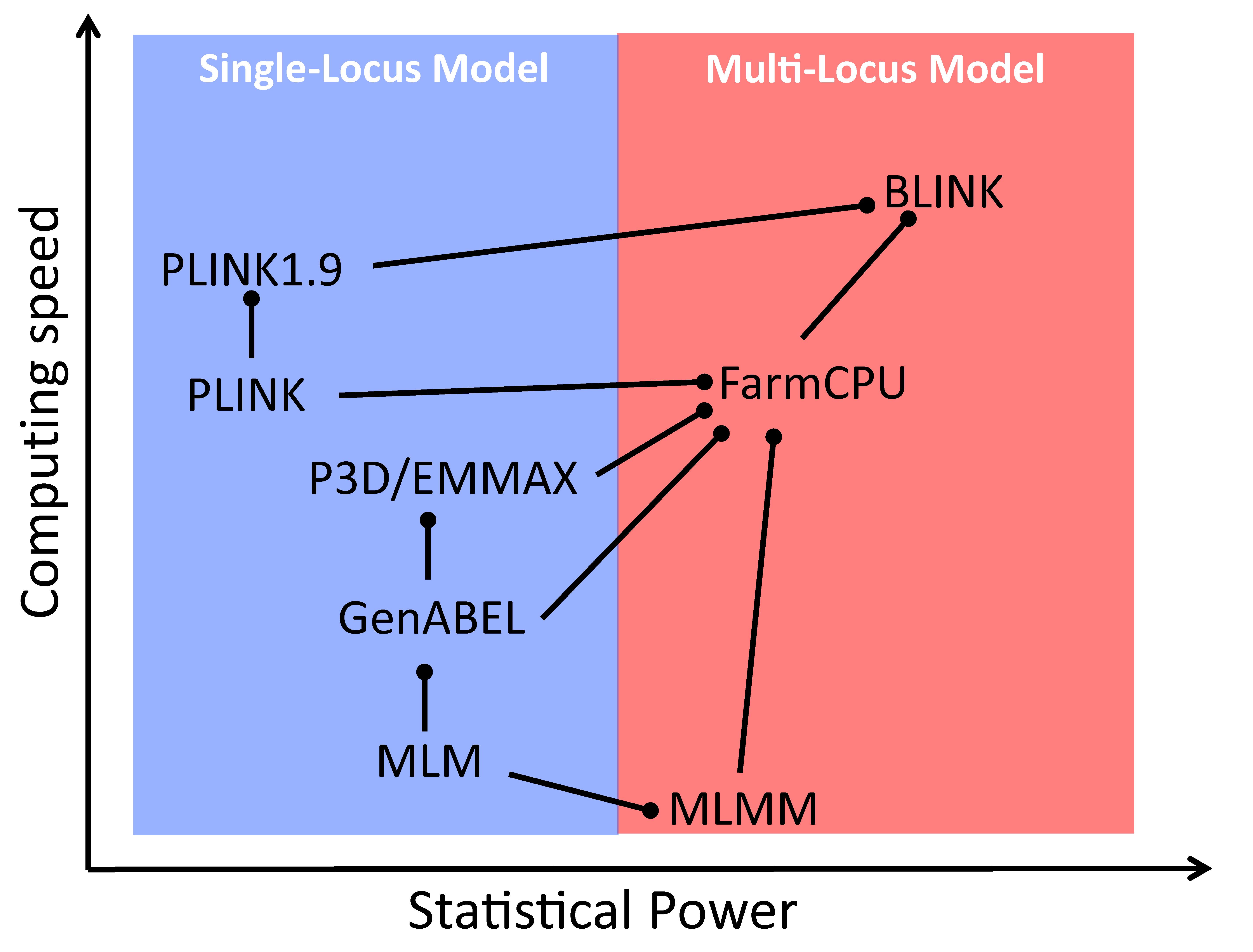
Comparison of GWAS models for statistical power and computing speed. The models are connected by lines with circle heads when direct comparisons exist in the literature. The models marked with circle heads have better power (vertical) or speed (horizontal). When power and speed are in contradiction, power is used. MLM: mixed linear model; CMLM: compressed MLM; ECMLM: enriched CMLM; SUPER: settlement of MLM under progressively exclusive relationship; FarmCPU: fixed and random model circulating probability unification; BLINK: Bayesian-information and linkage-disequilibrium iteratively nested keyway.
Background
The genome-wide association study (GWAS) is currently the primary method for mapping genes of interest and identifying genetic markers to predict the risk of human diseases and conduct marker-assisted selection for molecular breeding in animals and plants. Introduced in human genetic studies at the end of the last century, GWAS is a statistical inference of linkage disequilibrium (LD; please see Table S1 for all abbreviation definitions) caused by genetic linkage and many other factors, such as mutation, selection, and non-random mating [1–3]. Since GWAS aims to map genes based primarily on genetic linkage, excluding the influence of remaining factors during experimental design and data analysis is crucial [4,5].
Gene mapping depends on linkage analysis through crossing, especially in plants. As crossing is conducted in recent generations under controlled experiments, linkage analysis only needs to address type I errors. The corresponding drawback is the low mapping resolution due to limited recombination events over a small number of generations [6,7]. In contrast, GWAS relies on historical recombinations accumulated over many generations, resulting in high-resolution mapping at the gene level. Because genetic linkage is not the only reason for LD accumulated historically, GWAS must address both type I errors and spurious associations arising from population structure and selection [8–10].
With increasing marker density and complexity of enlarged plant samples, researchers face four roadblocks toward reporting their discoveries. The first roadblock is computing hardware and time. A genotype file of 100 GB is problematic for a computer with only 64 GB memory to analyze using R software packages without reading from the disk. For metabolic data, gene expression data, and electronic data with thousands of traits, computing time becomes a concern when analyzing a single trait takes several hours [11].
The second roadblock is statistical power, especially for small samples and traits with low heritability [12,13]. Although there are many statistical models and computing software packages with varied statistical power, researchers are not familiar with the majority and only use the ones they are familiar with, especially the ones developed earlier. Researchers gain confidence by seeing the overlaps with enlarged datasets using familiar statistical models and software, especially with published results, which is a cause of chain of false discoveries [14–16].
The third roadblock is to conduct GWAS properly. There are many factors that invite false positives, including phenotypic outliers and rare alleles of genetic markers in small samples [17]. Any combination of the three factors (outliers, rare allele, and small sample) could lead to false positives. The combination of outliers and rare alleles also leads to false positives even in large samples.
The fourth roadblock is to properly interpret phenotypic data, genotypic data, and association results. The most common mistake is inappropriately setting experiment-wise thresholds, leading to either hidden or false discoveries [18–20]. For simplicity, many researchers choose Bonferroni multiple test correction [21]. This threshold is over-conservative, especially for GWAS with dense markers where many markers are in close genetic linkage. The number of independent tests is far lower than the number of markers [22,23]. The opposite mistake is to underestimate the number of independent tests experiment-wise. When hundreds or thousands of traits are analyzed, a threshold of a single test type I error (e.g., 1%) divided by the number of independent markers generates far more false positives than expected from the single test type I error. The number of traits should be part of multipliers for the multiple test correction [24].
Our objective is to address these roadblocks so that researchers can conduct GWAS efficiently and produce truthful discoveries. First, we will provide an overview of statistical models and computing software to help readers decide whether to continue using familiar tools or explore advanced alternatives. Second, we will provide a step-by-step protocol showing how to properly conduct GWAS. Lastly, we will showcase a real publicly available rice dataset and demonstrate how to conduct GWAS and interpret phenotypic and genotypic data and analytical results. To allow readers to easily replicate our results and apply them to their own data, we limited our computing tools to only three software packages (BEAGLE [25], BLINK [26], and GAPIT [16,27,28]) for missing genotype imputation, GWAS, data management, analyses, and reports with publication-ready tables and figures.
Software and datasets
Model and software selection
Population structure is one of the most important causes of spurious association. Population structure matrix [4] or principal components [29] were incorporated as covariates to reduce spurious associations using general linear models (GLM) as implemented in PLINK [14], TASSEL [15], and GenABEL [30]. These software packages are intensively used due to computationally efficient GLM and popularity (Table 1). Multiple functions, such as file format conversion and linkage disequilibrium analysis, also contribute to their popularity [14,15].
Table 1. GWAS models and software implementations*
| Software | Year | Citations | GLM | MLM | CMLM | ECMLM | SUPER | MLMM | FarmCPU | BLINK |
| PLINK [14] | 2007 | 28141 | √ | |||||||
| TASSEL [15] | 2007 | 5930 | √ | √ | √ | |||||
| GenABEL [30] | 2007 | 2002 | √ | √ | ||||||
| EMMA [31] | 2008 | 1783 | √ | |||||||
| EMMAx [32] | 2010 | 1991 | √ | |||||||
| GCTA [33]# | 2011 | 5811 | √ | |||||||
| FaST-LMM [34] | 2011 | 1123 | √ | |||||||
| GEMMA [35] | 2012 | 2358 | √ | |||||||
| GAPIT [16,27,28] | 2012 | 1676 | √ | √ | √ | √ | √ | √ | √ | √ |
| MLMM [36] | 2012 | 787 | √ | |||||||
| FaST-LMM-Select [34] | 2012 | 351 | √ | √ | ||||||
| BOLT-LMM [13] | 2015 | 471 | √ | |||||||
| FarmCPU [37] | 2016 | 786 | √ | |||||||
| BLINK [26] | 2019 | 209 | √ | |||||||
| rMVP [17] | 2021 | 252 | √ | √ | √ | √ |
*Sorted by publication year and citations by year as of March 12, 2023. GWAS models include general linear model (GLM), mixed linear model (MLM) [5], compressed MLM (CMLM) [12], enriched CMLM (ECMLM) [38], settlement of MLM under progressively exclusive relationship (SUPER) [39], multiple loci mixed model (MLMM) [36], fixed and random model circulating probability unification (FarmCPU) [37], and Bayesian-information and linkage-disequilibrium iteratively nested keyway (BLINK) [26].
#equivalent to the approach of genomic best linear unbiased prediction (gBLUP) in genomic selection [40–42].
Besides population structure, another addition was introduced to control the unequal relatedness (kinship) among individuals within subpopulations using mixed linear models (MLM) [5]. Individuals’ total genetic effects are fitted as random effects with variance and covariance structure defined by the kinship derived from all genetic markers. Multiple algorithms were developed to improve the computing efficiency of MLM, including EMMA [31], P3D [12] (or EMMAx [32]), FaST-LMM [34], BOLT-LMM [13], and GEMMA [35]. These algorithms have the same statistical power as the regular MLM originally solved by the expectation and maximization algorithm [15]. MLM was also enhanced to improve statistical power by accounting for the confounding factor between testing markers and random individual total genetic effects, which causes false negatives. The models with improved statistical power include compressed MLM (CMLM) [12], enriched CMLM (ECMLM) [38], and FaST-LMM-Select [34] or SUPER [39]. FaST-LMM-Select and SUPER are equivalent. Some of the improved MLM models were implemented in software packages with multiple functions, including TASSEL [15] and GAPIT [16,27,28].
To further subtract the confounding between testing markers and the random individual genetic effects to improve statistical power, associated markers were introduced as covariates in the multiple loci mixed model (MLMM) [36]. The random individual genetic effect and testing markers were placed in a random effect model and in a fixed effect model separately (FarmCPU) [37]. Finally, the random individual genetic effects were completely removed in the BLINK model using GLM only [26]. BLINK uses two GLMs iteratively; one selects the associated markers as covariates with maximization of Bayesian information content, and the other tests markers one at a time with the selected associated markers as covariates. By doing so, BLINK not only retains GLM computing efficiency but also gains statistical power, higher than the other multiple loci models, including FarmCPU (Graphical overview). Some of the multiple loci models were implemented in software packages with multiple functions, including GAPIT [16,27,28] and RMVP [17].
Some of the models and software packages were compared for computation efficiency and statistical power against false discovery rates or type I errors (Graphical overview). GAPIT implemented the most models, from GLM, MLM, to SUPER for the single locus models and from MLMM, FarmCPU, to BLINK for the multiple loci models. The computing speed and statistical power can be examined by less than a handful of lines of R code (Box 1). The first three lines import the GAPIT source code, genotype data, and the genetic map from the GAPIT demo data (http://zzlab.net/GAPIT/data). The data contain 281 maize inbred lines and 3,093 single nucleotide polymorphisms (SNPs). The middle three lines set random seed and simulate phenotypes out of 40 SNPs sampled from the first five chromosomes as quantitative trait nucleotides (QTN) with heritability of 70%. The remaining chromosomes serve as a reference so that false positives can be easily identified. The last line calls GAPIT to conduct GWAS with seven models, including FarmCPU and BLINK. The execution takes approximately five minutes on a standard laptop. Some models consume more time than others. Users can assess the computing times of specific models by examining the result files, e.g., Manhattan plots, in the R working directory.
Box 1. R code to import GAPIT and genotype data, simulate phenotypes, and conduct GWAS
#Import GAPIT and demo data source("http://raw.githubusercontent.com/jiabowang/GAPIT/refs/heads/master/gapit_functions.txt") myGD=read.table(file="http://zzlab.net/GAPIT/data/mdp_numeric.txt",head=T) myGM=read.table(file="http://zzlab.net/GAPIT/data/mdp_SNP_information.txt",head=T) #Simultate QTNs on the first five chromosomes set.seed(99164) index1to5=myGM[,2]<6 mySim=GAPIT.Phenotype.Simulation(GD=myGD[,c(TRUE,index1to5)],GM=myGM[index1to5,], h2=.7, NQTN=40, QTNDist="normal") #GWAS with GAPIT using multiple models myGAPIT=GAPIT(Y=mySim$Y,GD=myGD,GM=myGM,PCA.total=3,QTN.position=mySim$QTN.position, model=c("GLM", "MLM", "CMLM", "SUPER", "MLMM", "FarmCPU", "BLINK")) |
GAPIT also combines all the Manhattan plots together for comparison (Figure S1). GLM identifies two QTNs based on the 5% type I error after Bonferroni multiple correction. MLM identifies one, CMLM identifies two, SUPER and MLMM identify seven, FarmCPU identifies eight, and BLINK identifies eleven. Users can replace the demo genotypes and genetic maps with their own, change the number of PCs, specify models, and conduct multiple replicates with different random seeds to achieve a more robust evaluation of the statistical power over different models on specific data sets.
Real case data
Rice 3000 genome project data (http://ricediversity.org/data/index.cfm) were used for real case analysis. This dataset includes 700K SNPs and 847 accessions published with the GWAS results of rice grain length [43]. The genotype data in PLINK format can be downloaded from http://ricediversity.org/data/sets_hydra/HDRA-G6-4-RDP1-RDP2-NIAS-2.tar.gz. The map file can be downloaded from http://ricediversity.org/data/sets_hydra/HDRA-G6-4-SNP-MAP.tar.gz. The phenotype data file can be downloaded from http://ricediversity.org/data/sets_hydra/phenoAvLen_G6_4_RDP12_ALL.tar.gz. The map version of genotype data is Rice Genome Project version 7. The genome position of known genes was searched from the phytozome database (https://phytozome-next.jgi.doe.gov/).
Procedure
文章信息
稿件历史记录
提交日期: Oct 16, 2024
接收日期: Mar 19, 2025
在线发布日期: Apr 3, 2025
出版日期: Apr 20, 2025
版权信息
© 2025 The Author(s); This is an open access article under the CC BY license (https://creativecommons.org/licenses/by/4.0/).
如何引用
Zuo, Z., Li, M., Liu, D., Li, Q., Huang, B., Ye, G., Wang, J., Tang, Y. and Zhang, Z. (2025). GWAS Procedures for Gene Mapping in Diverse Populations With Complex Structures. Bio-protocol 15(8): e5284. DOI: 10.21769/BioProtoc.5284.
分类
生物信息学与计算生物学
系统生物学 > 基因组学 > 全基因组关联分析
您对这篇实验方法有问题吗?
在此处发布您的问题,我们将邀请本文作者来回答。同时,我们会将您的问题发布到Bio-protocol Exchange,以便寻求社区成员的帮助。