

X-Ray Photon Correlation Spectroscopy, Microscopy, and Fluorescence Recovery After Photobleaching to Study Phase Separation and Liquid-to-Solid Transition of Prion Protein Condensates
结合X射线光子相关光谱、显微成像与荧光漂白恢复技术研究朊蛋白凝聚体的相分离及液-固转变过程
(*contributed equally to this work) 发布: 2025年04月20日第15卷第8期 DOI: 10.21769/BioProtoc.5277 浏览次数: 3847
评审: Marion HoggRama Reddy GoluguriRupam GhoshAnonymous reviewer(s)
参见作者原研究论文
The authors used this protocol in:

Nov 2023
Advertisement


Abstract
Biomolecular condensates are macromolecular assemblies constituted of proteins that possess intrinsically disordered regions and RNA-binding ability together with nucleic acids. These compartments formed via liquid-liquid phase separation (LLPS) provide spatiotemporal control of crucial cellular processes such as RNA metabolism. The liquid-like state is dynamic and reversible, containing highly diffusible molecules, whereas gel, glass, and solid phases might not be reversible due to the strong intermolecular crosslinks. Neurodegeneration-associated proteins such as the prion protein (PrP) and Tau form liquid-like condensates that transition to gel- or solid-like structures upon genetic mutations and/or persistent cellular stress. Mounting evidence suggests that progression to a less dynamic state underlies the formation of neurotoxic aggregates. Understanding the dynamics of proteins and biomolecules in condensates by measuring their movement in different timescales is indispensable to characterize their material state and assess the kinetics of LLPS. Herein, we describe protein expression in E. coli and purification of full-length mouse recombinant PrP, our in vitro experimental system. Then, we describe a systematic method to analyze the dynamics of protein condensates by X-ray photon correlation spectroscopy (XPCS). We also present fluorescence recovery after photobleaching (FRAP)-optimized protocols to characterize condensates, including in cells. Next, we detail strategies for using fluorescence microscopy to give insights into the folding state of proteins in condensates. Phase-separated systems display non-equilibrium behavior with length scales ranging from nanometers to microns and timescales from microseconds to minutes. XPCS experiments provide unique insights into biomolecular dynamics and condensate fluidity. Using the combination of the three strategies detailed herein enables robust characterization of the biophysical properties and the nature of protein phase-separated states.
Key features
• For FRAP in cells, we recommend using a spinning disk confocal microscope coupled with temperature and CO2 incubator.
• For fluorescence microscopy, we recommend simultaneously imaging differential interference contrast (DIC) (or phase contrast) and fluorescence channels to obtain morphological details of phase-separated structures.
• For XPCS, coherent X-ray beams, fast X-ray detectors in fourth and third synchrotron light sources, and X-ray free-electron lasers are required.
Keywords: Biomolecular condensates (生物大分子凝聚体)Graphical overview
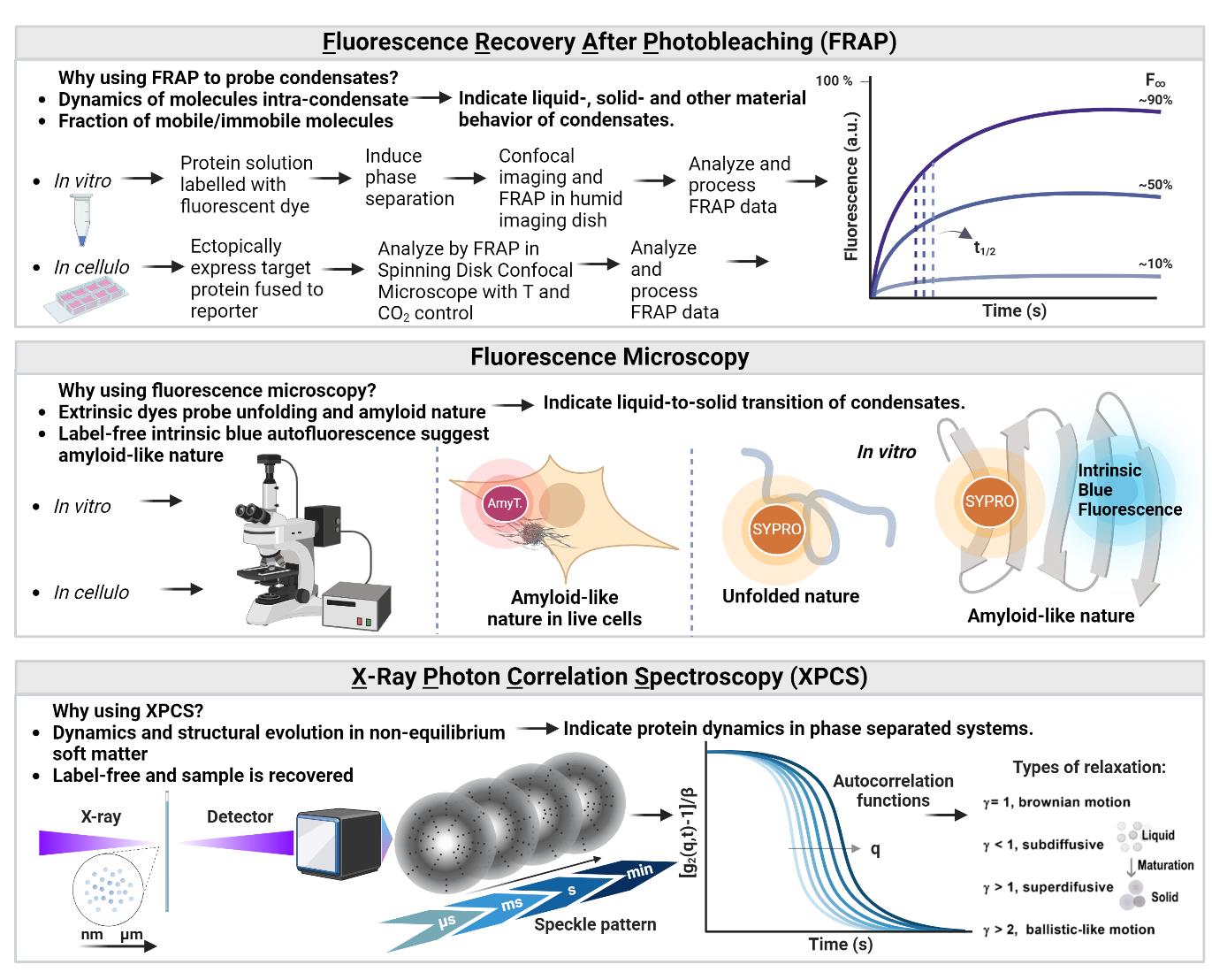
Biophysical methods to characterize biomolecular condensates. Top: Experiments using fluorescence recovery after photobleaching (FRAP) probe the mobility of proteins, RNAs, or other molecules composing the dense phase. The fraction of mobile molecules corresponds to the plateau fluorescence (F∞), and the kinetics of recovery are extracted from the half-time of maximum recovery (t1/2). These FRAP parameters are crucial to probe the material state of condensates that can behave as liquids, gels, soft glasses, and solids. Middle: Fluorescence microscopy approaches can inform on the structure of solid-like condensates. For example, SYPRO orange binds to hydrophobic residues exposed to solvent, indicating protein unfolding. AmyTracker 680 probes cross-β structures indicative of amyloid fold. Bottom: XPCS is a coherent scattering technique that probes dynamics in non-equilibrium systems. Monitoring the dynamics during LLPS is important to determine the biomolecular condensate state and droplet fluidity. Figure created in BioRender.com.
Background
The aggregation of the cellular prion protein (PrPC; Uniprot ID P04156) into the pathological scrapie PrP (PrPSc) leads to the development of prion diseases, including Creutzfeldt–Jakob disease in humans, and other fatal neurodegenerative disorders, with average survival time of one year after diagnosis, depending on the disease subtype. It is crucial to understand the mechanism by which PrPC, a monomeric protein that is ~50% disordered (N-terminal domain; residues 23–120) and ~50% globular (C-terminal domain; 120–230), misfolds into amyloids—highly ordered multimers enriched in cross-beta sheet structure—that are protease-resistant (PrPSc) and deposit in the brain (reviewed in [1]). In addition to classical theories of amyloid formation, a non-canonical pathway of misfolding seems to involve protein monomers or multimers in metastable biomolecular condensates, which are protein-rich membranelles assemblies [2,3]. Biomolecular condensates are formed by liquid-liquid phase separation and are driven by proteins enriched in intrinsic disorder and prion-like domains or low complexity sequences, as polar and aromatic residues establish multivalent weak intermolecular interactions that trigger condensation (reviewed in [4,5]).
Condensates display a myriad of functions across different cellular compartments. For example, cytosolic Tau condensates on the microtubule surface are suggested to regulate the movement of motors (reviewed in [6]), Golgi matrix proteins (e.g., Golgins and GRASPS) are suggested to organize the structure of Golgi by their phase separation property (reviewed in [7]), and nucleoid-associated proteins of E. coli compact DNA via phase separation, organizing sub-domains in nucleoids [8]. To understand the role of protein phase separation in cellular outcomes, as well as its relevance to aggregate formation, in vitro reconstituted systems that monitor protein dynamics within condensates, in combination with in cellulo approaches where condensation can be manipulated and quantitatively assessed, are required. Fluorescence recovery after photobleaching (FRAP) has become one of the most useful techniques to quantify the mobile vs. immobile fractions of biomolecules and their exchange between light and dense phases [9,10].
Here, we describe a systematic method to analyze the dynamics of condensates using the full-length PrP as a model. We have recently shown that the full-length PrP forms condensates in response to copper ions in vitro and at the cell–cell interface of live cells exposed to exogenous Cu2+. We first provide a standardized protocol using X-ray photon correlation spectroscopy (XPCS), a synchrotron technique that uses coherent X-rays to resolve the collective dynamics in concentrated protein systems. Because the dynamics of phase-separated systems display non-equilibrium behavior with length scales ranging from nanometers to microns and timescales from microseconds to minutes, XPCS can provide unique insights into biomolecular dynamics and condensate fluidity. Next, we detail strategies using fluorescence microscopy to gain insights into the folding state of proteins in condensates, utilizing extrinsic fluorescence such as SYPRO and AmyTracker 680 that probe unfolding and amyloids. Finally, we describe in vitro FRAP-optimized protocols to characterize reconstituted condensates using recombinant proteins fused to fluorescent reporters (e.g., Alexa 647). For FRAP in cells, we expressed PrPC fused to the enhanced yellow fluorescent protein (EYFP) in HEK293 and monitored FRAP dynamics upon exposure to copper ions in cell media. Using the combination of the three strategies detailed herein enables robust characterization of the biophysical properties and nature of phase-separated states.
Materials and reagents
Biological materials
1. Proteins:
a. Recombinant full-length murine prion protein (rPrP, residues 23–231) without any tag. PrP has an intrinsic ability to coordinate divalent transition metals in the octapeptide region (also termed octarepeats, OR) that we take advantage of to purify using Ni2+-affinity chromatography (explained in Section C) [11]. Mouse PrP has five ORs that can bind up to 4 copper ions, and two additional His in the N-terminal domain can also bind Cu2+, making it six sites for Cu2+
Note: Recombinantly expressed PrP (rPrP) at 70–100 μM is stored in low protein binding microcentrifuge tubes in ultrapure H2O at -20 °C for up to 6 months. We found that rPrP protein stability and solubility as well as secondary and tertiary structures are maintained using these conditions. In addition, rPrP does not phase-separate in H2O; checking this is essential, as LLPS-forming proteins cannot be stored in a condition where phase separation is favored.
b. rPrP labeled with Alexa Fluor 647 (Alexa Fluor® 647 carboxylic acid, succinimidyl ester) by formation of a stable dye-protein conjugate, as the reactive dye contains a succinimidyl ester moiety that reacts with primary amines of proteins such as the N-terminus and the side-chain of lysine residues (Thermo Fisher, catalog number: A20173) (see [12] for the labeling procedure and consult the manufacturer’s manual)
2. Plasmids:
a. pET-41, in which mouse PrP cDNA (corresponding to amino acid residues 23–230, mature protein) was cloned into NdeI and HindIII sites (original HisTag in the plasmid was removed) for expression in Escherichia coli (refer to Section A)
b. pEYFP-N1 for mammalian expression of PrPC-EYFP-GPI (kindly gifted by Marilene H. Lopes, USP, Brazil) (refer to Section J)
c. pCR3-EYFP-GPI (DAF) for mammalian expression of YFP-GPI (kindly gifted by Daniel Legler, Universität Konstanz, Germany) (refer to Section J)
3. Human embryonic kidney cell line (HEK293 cells) (ATCC, CRL-1573) (refer to Sections J, K, L, and N)
4. Escherichia coli BL21 (DE3) (Thermo Scientific, catalog number: EC0114) (refer to Section A)
Reagents
1. Ultrapure water, treated by reverse osmosis, filtered, and deionized (resistivity of 18.2 MΩ·cm and pH 6.9 at 25 °C)
2. Copper (II) chloride dihydrate (CuCl2·2H2O) (Sigma-Aldrich, catalog number: 307483)
3. 30% (w/v) hydrogen peroxide (H2O2) (Millipore, catalog number: 88597)
4. 4-(2-Hydroxyethyl)piperazine-1-ethanesulfonic acid (HEPES) (C8H18N2O4S) (Sigma-Aldrich, catalog number: V900477)
5. Potassium chloride (KCl) (Sigma-Aldrich, catalog number: P3911)
6. Potassium hydroxide (KOH) (Sigma-Aldrich, catalog number: 484016)
7. Sodium chloride (NaCl) (Sigma-Aldrich, catalog number: S1679)
8. Calcium chloride dihydrate (CaCl2·2H2O) (Sigma-Aldrich, catalog number: V900269)
9. Magnesium chloride hexahydrate (MgCl2·6H2O) (Sigma-Aldrich, catalog number: M2670)
10. Polyethylene glycol (PEG) 4000 (Sigma-Aldrich, catalog number: 81240)
11. Alexa Fluor® 647 Protein Labeling kit (Thermo Fisher, catalog number: A20173)
12. Hydrochloric acid (HCl) (Sigma-Aldrich, catalog number: 30721)
13. Sodium hydroxide (NaOH) (Sigma-Aldrich, catalog number: S5881)
14. Phosphate-buffered saline (PBS) (Thermo Fisher, catalog number: 10010001)
15. Recombinant PrP expression and purification (Sections B and C)
a. 2-amino-2-(hydroxymethyl)-1,3-propanediol (Tris) (C4H11NO3) (Sigma-Aldrich, catalog number: 252859)
b. Ethylenediaminetetraacetic acid (EDTA) (C10H14N2Na2O8·2H2O) (Sigma-Aldrich, catalog number: E4884)
c. Disodium hydrogen phosphate (Na2HPO4) (Sigma-Aldrich, catalog number: S9763)
d. α-D-Glucopyranosyl β-D-fructofuranoside (sucrose) (C12H22O11) (Sigma-Aldrich, catalog number: S8501)
e. Lysozyme from chicken egg white (Sigma-Aldrich, catalog number: L6876)
f. CelLytic B cell lysis reagent (Sigma-Aldrich, catalog number: B7435)
g. Sodium dihydrogen phosphate (NaH2PO4) (Sigma-Aldrich, catalog number: S0751)
h. UltraPure guanidine hydrochloride (CH6ClN3) (Invitrogen, catalog number: 15502016)
i. 1,3-Diaza-2,4-cyclopentadiene (imidazole) (C3H4N2) (Sigma-Aldrich, catalog number: I202)
j. Agar (Becton Dickinson Bioscience, catalog number: 214010)
k. Luria-Bertani (LB) broth (Becton Dickinson Bioscience, catalog number: 244620)
l. Super optimal broth (SOC) (Sigma-Aldrich, catalog number: S1797)
m. Phenylmethanesulfonyl fluoride (PMSF) (C7H7FO2S) (Sigma-Aldrich, catalog number: P7626)
n. HisTrap HP, 5 mL (Cytiva, catalog number: 17524802)
o. SnakeSkin dialysis tubing 10 K MWCO (Thermo Scientific, catalog number: 68100)
p. Triton X-100 (Sigma-Aldrich, catalog number: X100)
q. Colloidal Coomassie G-250 stain for protein polyacrylamide gels (Bio-Rad, catalog number: 1610803)
16. Media for cell culture (Sections J, L, K, and N)
a. Dulbecco’s modified Eagle’s medium (DMEM) (Sigma-Aldrich, catalog number: D5546)
b. Fetal bovine serum (FBS) (Gibco, catalog number: A5670801)
c. Penicillin-Streptomycin 100× (Sigma-Aldrich, catalog number: P4333)
17. Reagents for transfection for in cellulo FRAP experiments (Sections J–L)
a. Opti-MEM I (Gibco, catalog number: 31985062)
b. Lipofectamine 2000 (Invitrogen, catalog number: 11668027)
18. Extrinsic dyes for fluorescence microscopy (Sections H and N)
a. SYPRO orange (5,000× stock in DMSO) (Sigma-Aldrich, catalog number: S5692)
b. AmyTracker 680 (Ebba Biotech AB)
19. Standard for calibration of q-angle for XPCS experiments (Sections E and F)
a. Silver(I) behenate (Thermo Scientific Chemicals, catalog number: 15452307)
Solutions
1. STE buffer (see Recipes)
2. Buffered sucrose (see Recipes)
3. Buffer A (denaturing buffer pH 8.0) (see Recipes)
4. Buffer B (refolding buffer pH 8.0) (see Recipes)
5. Elution buffer pH 5.0 (see Recipes)
6. 2× Physiological-like buffer (PhysB) pH 7.2 (see Recipes)
7. CuCl2, 0.1 M (see Recipes)
8. 3% (or 0.88 M) H2O2 (see Recipes)
9. rPrP sample (see Recipes)
10. rPrP+CuCl2 sample (see Recipes)
11. rPrP+CuCl2+H2O2 sample (see Recipes)
12. Media for cell culture (complete DMEM) (see Recipes)
Recipes
1. STE buffer, pH 8 (100 mL)
| Reagent | Final concentration | Quantity or Volume |
|---|---|---|
| Tris | 50 mM | 0.6056 g |
| NaCl | 10 mM | 0.0584 g |
| EDTA | 5 mM | 0.1861 g |
a. Dissolve the solids in ~80 mL of ultrapure H2O and stir until completely dissolved using a magnetic stirrer.
b. Monitor the pH of the solution (it should be ~7.0–7.5) and adjust to 8 by carefully adding NaOH.
c. Adjust the final volume to 100 mL.
d. Filter-sterilize the solution using a 0.22 μm syringe filter.
e. Store the prepared buffer at 4 °C for up to 1 month.
Note: It is recommended to always use freshly prepared buffers to ensure optimal performance.
2. Buffered sucrose, pH 7.2 (50 mL)
| Reagent | Final concentration | Quantity or Volume |
|---|---|---|
| Na2HPO4 | 20 mM | 0.14196 g |
| NaCl | 20 mM | 0.0292 g |
| EDTA | 5 mM | 0.0931 g |
| Sucrose | 25% (m/v) | 12.5 g |
a. Dissolve the solids in ~30 mL of ultrapure H2O and stir until completely dissolved using a magnetic stirrer.
b. Monitor the pH of the solution (it should be ~7.5–8.0) and adjust to 7.2 by carefully adding HCl.
c. Adjust the final volume to 50 mL with ultrapure H2O.
d. Store the prepared buffer at 4 °C for up to 1 month.
Note: Filtration is not necessary for this buffer due to the high concentration of sucrose, which increases viscosity. Ensure the solution is fully homogeneous and all components are completely dissolved before verifying the pH.
3. Buffer A (denaturing buffer) pH 8.0 (500 mL)
| Reagent | Final concentration | Quantity or Volume |
|---|---|---|
| Ultrapure guanidine | 6 M | 286.59 g |
| Tris | 10 mM | 0.6056 g |
| Na2HPO4 | see note* | 6.7241 g |
| NaH2PO4 | see note* | 0.3184 g |
a. Dissolve Na2HPO4 and NaH2PO4 in ultrapure water and stir until completely dissolved using a magnetic stirrer.
b. Add Tris to the solution and continue stirring until fully dissolved.
c. Add ultrapure guanidine hydrochloride (GdnHCl) and continue stirring until the powder is completely dissolved.
d. Monitor the pH of the solution. If necessary, adjust the pH carefully to 8.0 using HCl or NaOH.
e. Adjust the final volume to 500 mL with ultrapure water.
f. Filter-sterilize the solution using a 0.22 μm syringe filter to ensure sterility.
g. Store the prepared buffer at 4 °C for up to 1 month.
Notes:
1. Ultrapure guanidine (purity ≥99%) is required to avoid impurities that could interfere with the protein purification process.
2. Guanidine is highly hygroscopic and contributes significantly to the final volume.
*Note: Sodium phosphate buffer (monobasic + dibasic) has a final concentration of 100 mM.
4. Buffer B (refolding buffer) pH 8.0 (600 mL)
| Reagent | Final concentration | Quantity or Volume |
|---|---|---|
| Tris | 10 mM | 0.7268 g |
| Na2HPO4 | see note* | 8.0662 g |
| NaH2PO4 | see note* | 0.3815 g |
a. Dissolve Na2HPO4 and NaH2PO4 in ultrapure water and stir until completely dissolved using a magnetic stirrer.
b. Add Tris to the solution and continue stirring until fully dissolved.
c. Monitor the pH of the solution. If necessary, adjust the pH carefully to 8.0 using HCl or NaOH.
d. Adjust the final volume to 600 mL with ultrapure water.
e. Filter-sterilize the solution using a 0.22 μm syringe filter to ensure sterility.
f. Store the prepared buffer at 4 °C for up to 1 month.
*Note: Sodium phosphate buffer (monobasic + dibasic) has a final concentration of 100 mM.
5. Elution buffer pH 5.0 (500 mL)
| Reagent | Final concentration | Quantity or Volume |
|---|---|---|
| Imidazole | 500 mM | 17.02 g |
| NaH2PO4 | 100 mM | 6.0 g |
a. Dissolve NaH2PO4 in ultrapure water and stir until completely dissolved using a magnetic stirrer.
b. Add imidazole to the solution and continue stirring until fully dissolved.
c. Monitor the pH of the solution using a calibrated pH meter. If necessary, adjust the pH carefully to 5.0 using HCl or NaOH.
d. Adjust the final volume to 500 mL with ultrapure water.
e. Filter-sterilize the solution using a 0.22 μm syringe filter to ensure sterility.
f. Store the prepared buffer at 4 °C for up to 1 month.
Note: A significant volume of HCl may be required to reach this pH due to the buffering capacity of imidazole.
6. 2× Physiological-like buffer (PhysB) pH 7.2 (100 mL)
| Reagent | Final concentration (2×) | Quantity or Volume |
|---|---|---|
| HEPES | 20 mM | 0.4766 g |
| KCl | 240 mM | 1.7894 g |
| NaCl | 10 mM | 0.5844 g |
| CaCl2·2H2O | 300 μM | 0.0441 g |
| MgCl2·6H2O | 10 mM | 2.033 g |
| PEG 4000 | 120 mg/mL | 12 g |
| Ultrapure H2O | n/a | to 100 mL |
| Total | n/a | 100 mL |
a. Dissolve the solids in ~80 mL of ultrapure H2O and stir until complete dissolution using a magnetic stirrer.
b. Monitor the pH of the solution (should be acidic, ~5.5) and adjust to 7.2 by carefully adding KOH flakes (do not use NaOH since K+ is prevalent over Na+ in the cellular milieu; see Theillet et al. [13]).
c. Complete the volume to 100 mL.
d. Filter-sterilize using a 0.22 μm syringe filter.
e. Store at 4 °C for up to 1 month or freeze at -20 °C for up to 6 months.
f. Equilibrate the buffer for at least 30 min at room temperature before preparing samples for experiments.
7. CuCl2 0.1 M
| Reagent | Final concentration | Quantity or Volume |
|---|---|---|
| CuCl2·2H2O | 100 mM | 0.85 g |
| Ultrapure H2O | n/a | 49.1 mL |
| Total | n/a | 50 L |
a. Using a CuCl2 powder stored in a sealed container kept inside a desiccator (hygroscopic), weigh the corresponding amount.
b. Completely dissolve the CuCl2 powder.
c. Filter-sterilize and keep at room temperature.
8. 3% (or 0.88 M) H2O2
| Reagent | Final concentration | Quantity or Volume |
|---|---|---|
| Ultrapure H2O | n/a | 450 μL |
| 8.8 M H2O2 | 0.88 M | 50 μL |
| Total | n/a | 500 μL |
Add components in this order in a microcentrifuge tube (1.5 mL capacity).
Note: H2O2 decomposes quickly; make this diluted solution just before preparing the sample. Once open, keep the 30% w/v H2O2 stock container at 4 °C for up to 6 months.
9. rPrP sample
| Reagent | Final concentration | Quantity or Volume |
|---|---|---|
| Ultrapure H2O | n/a | 71 μL |
| 2× physiological buffer (Recipe 6) | 1× | 250 μL |
| rPrP 70 μM | 25 μM | 179 μL |
| Total | n/a | 500 μL |
Add components in this order in a low protein binding microcentrifuge tube.
10. rPrP+CuCl2 sample
| Reagent | Final concentration | Quantity or Volume |
|---|---|---|
| Ultrapure H2O | n/a | 21 μL |
| 2× Physiological buffer (Recipe 6) | 1× | 250 μL |
| rPrP 70 μM | 25 μM | 179 μL |
| CuCl2 2 mM | 200 μM | 50 μL |
| Total | n/a | 500 μL |
Add components in this order in a low protein binding microcentrifuge tube.
11. rPrP+CuCl2+H2O2 sample
| Reagent | Final concentration | Quantity or Volume |
|---|---|---|
| Ultrapure H2O | n/a | 15.3 μL |
| 2× Physiological buffer (Recipe 6) | 1× | 250 μL |
| rPrP 70 μM | 25 μM | 179 μL |
| CuCl2 2 mM | 200 μM | 50 μL |
| H2O2 (3% w/v or 0.98 M) | 10 mM | 5.7 μL |
| Total | n/a | 500 μL |
Add components in this order in a low protein binding microcentrifuge tube.
Note: H2O2 decomposes quickly. Therefore, to have a 3% w/v (or 0.88 M) H2O2 solution, make a 1:10 dilution of 30% w/v H2O2 in ultrapure H2O just before preparing the sample (e.g., 50 μL of H2O2 + 450 μL of H2O) (Recipe 8). Once open, keep the 30% w/v H2O2 stock container at 4 °C for up to 6 months.
12. Media for cell culture (complete DMEM)
| Reagent | Final concentration | Quantity or Volume |
|---|---|---|
| DMEM | n/a | 445 mL |
| FBS | 10% | 50 mL |
| Penicillin/Streptomycin 100× | 1% | 5 mL |
| Total | n/a | 500 mL |
Filter-sterilize using a 0.22 μm membrane, store at 4 °C, and prewarm at 37 °C before culturing HEK293 cells.
Laboratory supplies
1. XPCS measurements:
a. Silanized quartz capillary, 1.5 mm outer diameter, wall thickness 0.01 mm (Hampton Research, catalog number: HR6-128)
b. Disposable syringe, 1 mL
c. 1.5 mL microcentrifuge protein LoBind tubes (Eppendorf, catalog number: 0030108116)
2. Imaging chambers:
a. 35 × 10 mm diameter with a hole punched and 1.33 cm2 area glass coverslip (SPL, catalog number: 200350)
b. μ-slide 8-well confocal slides with lid (Ibidi, catalog number: 80806-90)
c. Coverslips #1 thickness size 22 × 22 mm (Knittel glass, catalog number: VD12222Y100A), microscope slides size 76 × 26 mm (Knittel glass, catalog number: VA21100001FKB), and double-sided tape (3-M Scotch 665-C, 19 mm × 32.9 m)
Equipment
1. XPCS beamline at a synchrotron facility. We used the Cateretê beamline at the Brazilian Synchrotron Light Laboratory (Sirius) [14]. The beamline parameters of the XPCS experiments are detailed in [12].
2. Confocal line-scanning inverted microscope (Carl Zeiss, model: LSM 710) equipped with a 100× objective (oil-immersion, NA 1.46, Carl Zeiss)
3. Confocal spinning disk inverted microscope (Nikon, model: Eclipse-Ti CSU-X) equipped with a 60× objective (oil-immersion, 60×, plan Apo, oil, NA 1.4, Nikon), perfect focus system (PFS), and coupled with temperature, humidity, and CO2 hypoxia incubator (On Stage Incubator, Okolab)
4. Fluorescence microscope (Leica, model: LMD 7) equipped with a 100× objective (Leica Microsystems, model: oil-immersion, NA 1.25)
5. Centrifuge (Hitachi, model: Himac CR22 GII)
6. Centrifuge (Heraeus, model: Megafuge 8R)
7. Spectrophotometer (Shimadzu, model: UV mini-1240)
8. Water bath (Novatecnica)
9. Sonicator (Sonics & Materials, model: VCX 130)
10. Thermal mixer (Eppendorf, model: ThermoMixer F1.5)
11. Incubator shaker (New Brunswick Scientific, model: Excella E24 Incubator Shaker Series)
12. Incubator (Quimis)
13. ÄKTAprimeTM plus (GE Healthcare)
Software and datasets
1. Fiji (Image J) (https://imagej.net/software/fiji/downloads access date July 1, 2024)
2. GraphPad Prism 8.1.1 (https://www.graphpad.com access date July 1, 2024)
3. Excel (Microsoft)
4. XPCS data analysis Python package developed in-house for the calculation of the autocorrelation from the scattering intensity. The software generates multi-tau, one-time, and two-time g2 modes based on the method described by [15]. The temporal autocorrelation function for a set of pixels in a region with an average wavevector q [q = (4π/λ) sin(θ/2) with θ the scattering angle] is given by the one-time correlation
5. SAXS data analysis: SAXS patterns were obtained from the averaged XPCS dataset using the PyFAI software package (https://www.esrf.fr/UsersAndScience/Publications/Highlights/2012/et/et3)
Procedure
文章信息
稿件历史记录
提交日期: Oct 24, 2024
接收日期: Mar 6, 2025
在线发布日期: Mar 26, 2025
出版日期: Apr 20, 2025
版权信息
© 2025 The Author(s); This is an open access article under the CC BY-NC license (https://creativecommons.org/licenses/by-nc/4.0/).
如何引用
Readers should cite both the Bio-protocol article and the original research article where this protocol was used:
- Do Amaral, M. J., Passos, A. R., Mohapatra, S., Freire, M. H., Wegmann, S. and Cordeiro, Y. (2025). X-Ray Photon Correlation Spectroscopy, Microscopy, and Fluorescence Recovery After Photobleaching to Study Phase Separation and Liquid-to-Solid Transition of Prion Protein Condensates. Bio-protocol 15(8): e5277. DOI: 10.21769/BioProtoc.5277.
- Do Amaral, M. J., Mohapatra, S., Passos, A. R., Lopes da Silva, T. S., Carvalho, R. S., da Silva Almeida, M., Pinheiro, A. S., Wegmann, S. and Cordeiro, Y. (2023). Copper drives prion protein phase separation and modulates aggregation. Sci Adv. 9(44): eadi7347. https://doi.org/10.1126/sciadv.adi7347
分类
生物物理学 >
生物物理学 > 显微技术
生物化学 > 蛋白质 > 活性
您对这篇实验方法有问题吗?
在此处发布您的问题,我们将邀请本文作者来回答。同时,我们会将您的问题发布到Bio-protocol Exchange,以便寻求社区成员的帮助。