

An Open-source Python Tool for Traction Force Microscopy on Micropatterned Substrates
用于微图案化基质牵引力显微分析的开源Python工具
发布: 2025年01月05日第15卷第1期 DOI: 10.21769/BioProtoc.5156 浏览次数: 1680
评审: Marc-Antoine SaniDjamel Eddine ChafaiAnonymous reviewer(s)
参见作者原研究论文
The authors used this protocol in:

Aug 2023
Advertisement


Abstract
Cell-generated forces play a critical role in driving and regulating complex biological processes, such as cell migration and division and cell and tissue morphogenesis in development and disease. Traction force microscopy (TFM) is an established technique developed in the field of mechanobiology used to quantify cellular forces exerted on soft substrates and internal mechanical tissue stresses. TFM measures cell-generated traction forces in 2D or 3D environments with varying mechanical and biochemical properties. This technique involves embedding fiducial markers in the substrate, imaging substrate deformations caused by the cells, and using mathematical models to infer forces. This protocol compiles procedures from various previously published studies and software packages and describes how to perform TFM on 2D micropatterned substrates. Although not the focus of this protocol, the methods and software packages shown here also allow to perform monolayer stress microscopy (MSM), a method to calculate internal mechanical stress within the cells by modeling them as a thin plate with linear and homogeneous material properties. TFM and MSM are non-invasive methods capable of yielding spatially and temporally resolved force and stress maps with high throughput. As such, they enable the generation of rich datasets, which can provide valuable insights into the roles of cell-generated forces in various physiological and pathological processes.
Key features
• TFM and MSM protocol for 2D micropatterned polyacrylamide substrates, from sample preparation over imaging to data analysis with provided code.
• Sample preparation method is based on Tseng et al. [1].
• TFM analysis is done with Python custom code and is optimized for batch analysis of movies.
• MSM analysis is done with pyTFM from Bauer et al. [2].
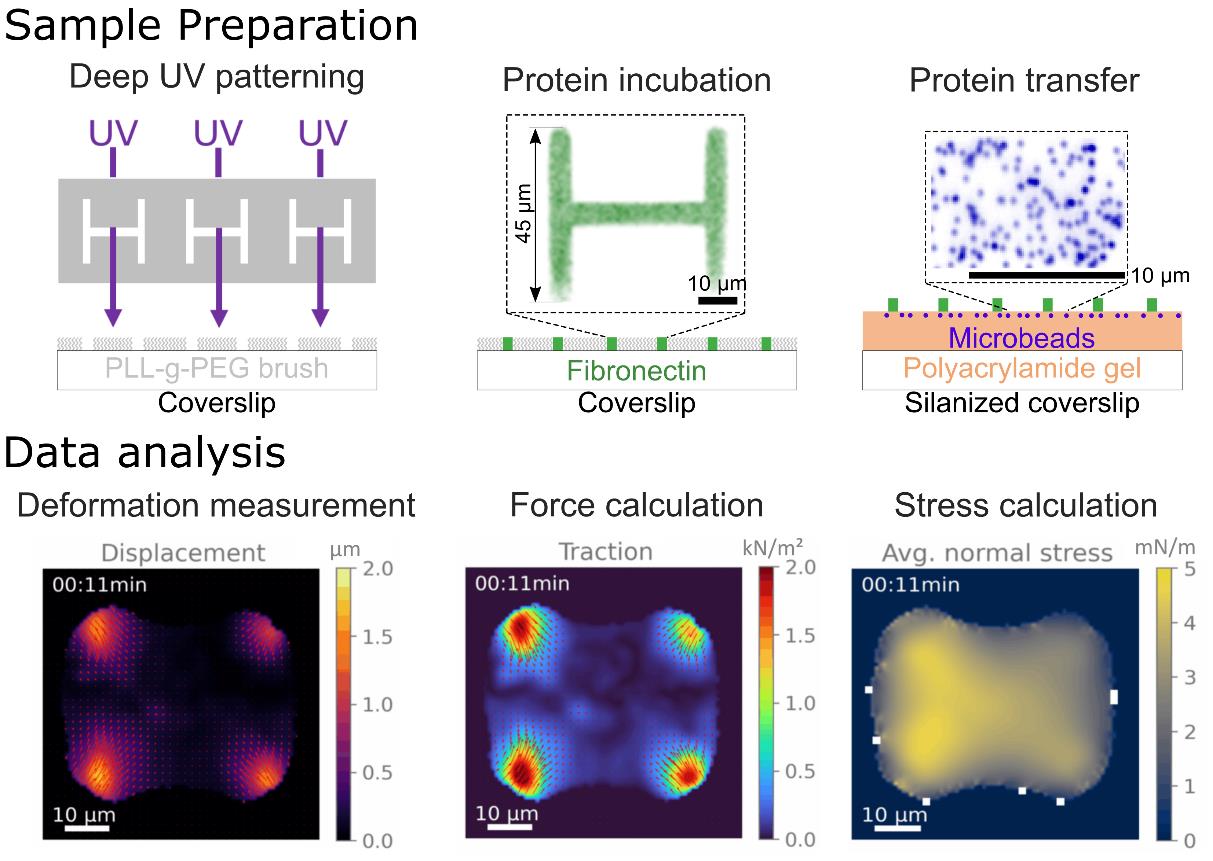
Keywords: Traction force microscopy (牵引力显微技术)Graphical overview
Background
This protocol combines micropatterning, traction force microscopy (TFM), and monolayer stress microscopy (MSM), well-established techniques in mechanobiology, each with a rich history and extensive literature. As such, everything described in this protocol has been used and published by many scientists in the past. However, there is a lack of a comprehensive protocol integrating all three, spanning from sample preparation to data analysis, which this work aims to address.
Micropatterning is a tool that allows the imposition of geometrical boundary conditions onto cells by depositing adhesive proteins onto a substrate in specific spots. This tool has led to significant discoveries, showing that geometrical parameters are important in regulating complex biological processes, such as apoptosis [3], differentiation [4], or multicellular organization [5]. To combine micropatterning with TFM, Wang et al. developed a PDMS stencil-based protocol [6]. Later, Tseng et al. developed a photolithography-based method for micropatterned soft substrates, which the protocol here is based on [1].
The foundational study for TFM was published in 1980 [7], pioneering the use of soft substrates to visualize cell-generated traction forces, where the authors placed fibroblasts on a thin silicone sheet, which then showed visible wrinkling caused by cell-generated traction forces. A major improvement of this method consisted of visualizing the deformation of the substrate through fiducial markers, enabling detailed measurements of deformation maps of the substrates. The first studies using these improvements showed the first estimation of traction force maps for keratocytes [8] and fibroblasts [9].
The calculation of the traction force maps from the deformation maps is mathematically and computationally complicated due to the ill-posed nature of the problem. A first solution was proposed by Dembo et al. [10] and then, in a much more computationally efficient way, by Butler et al. [11]. For a more detailed review of the mathematical and computational foundations of TFM, see [12].
TFM primarily examines cell–substrate interactions, lacking insights into cell–cell interactions in multicellular systems. While simple force balance arguments suffice for cell doublets [13,14], more complex systems necessitate advanced approaches. This led to the development of monolayer stress microscopy (MSM) by Tambe et al. [15], which models cell monolayers as thin plates with homogeneous, linear material properties. Detailed discussions on assumptions and limitations are available [16]. Various researchers have independently developed solutions based on the same physical formulation of the problem [2,17,18].
Most scientists who publish TFM and/or MSM data develop their own analysis code, which is usually available only upon request. This requires significant technical expertise, which slows down the wide adoption of this technique in labs with a stronger focus on biological questions. For TFM, a wide variety of freely available analysis code now exists in the literature, such as Cellogram for reference-free TFM [19], TFMLAB for 4D TFM [20], pyTFM [2], Han Lab’s TFM [21], or JEasyTFM and iTACS for standard 2D TFM [22, 23]. For MSM, pyTFM by Bauer et al. and iTACS by Nguyen et al. are freely available [2, 23].
In order to cater to our specific TFM analysis needs, we developed our own Python TFM code, which is available at https://github.com/ArturRuppel/batchTFM. It is completely open-source and optimized for batch analysis of movies. It relies on numerous open-source Python packages, such as numpy and scipy, and most notably, relies on pyTFM for the MSM calculations.
Materials and reagents
Biological materials
1. Cell type of interest, opto-MDCK cells in our case. Wildtype MDCK cells were kindly provided by Prof. Yasuyuki Fujita, University of Kyoto, and then genetically modified by Dr. Manasi Kelkar and Dr. Guillaume Charras
Reagents
1. Adhesion protein of interest (usually fibronectin; Sigma-Aldrich, catalog number: F1141)
2. Fluorescent protein of choice (usually fibrinogen conjugated with, e.g., Alexa 546; Thermo Fisher, catalog number: F13192)
3. Dulbecco’s modified Eagle medium (DMEM) (Thermo Fisher, catalog number: 11965092)
4. Fetal bovine serum (FBS) (Thermo Fisher, catalog number: A5256801)
5. Penicillin-streptomycin, 5,000 U/mL (pen/strep) (Thermo Fisher, catalog number: 15070063)
6. Trypsin 2.5% (Thermo Fisher, catalog number: 15090046)
7. Ethylenediaminetetraacetic acid (EDTA) 0.5M (Thermo Fisher, catalog number: AM9260G)
8. Sterile phosphate-buffered saline (PBS) (Sigma-Aldrich, catalog number: 806552)
9. 4-(2-hydroxyethyl)-1-piperazineethanesulfonic acid (HEPES) (Thermo Fisher, catalog number: A14777.30)
10. Sodium bicarbonate (Sigma-Aldrich, catalog number: PHR3591)
11. Poly(L-lysine)-g-poly(ethylene glycol) (PLL-g-PEG) [SuSoS, catalog name: PLL(20)-g[3.5]- PEG(5)]
12. 2% Bis-acrylamide solution (Sigma-Aldrich, catalog number: M1533)
13. 40% Acrylamide solution (Sigma-Aldrich, catalog number: A4058)
14. Tetramethylethylenediamine (TEMED) (Sigma-Aldrich, catalog number: T9281)
15. Ammonium persulfate (APS) (Sigma-Aldrich, catalog number: A3678)
16. FluoSpheres, carboxylate-modified (e.g., dark red; Thermo Fisher, catalog number: F8807)
17. Bind silane (Sigma-Aldrich, catalog number: M6514)
18. 99.8% Ethanol (Thermo Fisher, catalog number: 445730025)
19. 99.7% Acetic acid (Sigma-Aldrich, catalog number: 695092)
20. Isopropanol (Fisher, catalog number: BP2618-1)
21. 96% ethanol (Carlo Erba, catalog number: 308646)
Solutions
1. 100 mM sodium bicarbonate, prepared with MilliQ water
2. 10 mM HEPES buffer, pH 7.4, prepared with MilliQ water and pH adjusted with NaOH
3. 10% acetic acid, diluted with MilliQ water
4. Cell culture medium (see Recipes)
5. Trypsinization solution (see Recipes)
6. 0.1 g/L PLL-g-PEG solution (see Recipes)
7. Polyacrylamide premix (see Recipes)
8. Silanization solution (see Recipes)
Recipes
1. Cell culture medium
Prepare in a sterile hood and then store in the fridge.
| Reagent | Final concentration | Volume |
|---|---|---|
| DMEM | 89% | 445 mL |
| FBS | 10% | 50 mL |
| Pen/strep | 1% | 5 mL |
| Total | 500 mL |
2. Trypsinization solution
Prepare several aliquots in a sterile hood and then store in the freezer. Aliquots in use can be stored in the fridge for a few weeks.
| Reagent | Final concentration | Volume |
|---|---|---|
| Trypsin 2.5% | 0.25% | 1 mL |
| EDTA 0.5M | 0.5mM | 0.01 mL |
| MilliQ water | 8.99 mL | |
| Total | 10 mL |
3. 0.1 g/L PLL-g-PEG solution
Filter the solution through a 0.2 μm filter and store the aliquots in the freezer. Aliquots in use can be stored in the fridge and should be used within ~10 days.
| Reagent | Final concentration | Volume |
|---|---|---|
| PLL-g-PEG | 1 mg | 0.1 g/L |
| HEPES buffer 10mM pH 7.4 | 10mM | 10 mL |
| Total | 10 mL |
4. Polyacrylamide premix
The exact recipe depends on the desired rigidity of the gel and can be found in [23]. Here, we provide the recipe for 20 kPa gels, also taken from [23]. Prepare in the fume hood. Can be stored in the fridge for years.
| Reagent | Final concentration | Volume |
|---|---|---|
| 40% Acrylamide solution | 8% | 2 mL |
| 2% Bis-acrylamide solution | 0.264% | 1.32 mL |
| MilliQ water | 6.68 mL | |
| Total | 10 mL |
5. Silanization solution
Prepare under the fume hood and discard after use in appropriate chemical waste containers.
| Reagent | Final concentration | Volume |
|---|---|---|
| Bind silane | 0.35% | 35 μL |
| 10% acetic acid | 0.324% | 325 μL |
| 99.8% ethanol | 9.64 mL | |
| Total | 10 mL |
Laboratory supplies
1. Borosilicate coverslips (32 and 25 mm) (VWR, catalog number: 631-0162 and 631-0171)
2. Coverslip cell chamber (e.g., from Aireka Cells or custom-made in a workshop. Technical drawings are available upon request)
3. Nitrogen spray gun (VWR, catalog number: ENTE421-42-11)
4. Tweezers (VWR, catalog number: 232-1220)
5. Squirt bottles (VWR, catalog number: 89141-044)
6. Photomask (Toppan)
7. Dish soap (argos, catalog number: 4202)
8. Kimwipe (Sigma, catalog number: Z671584)
9. Scalpel (Sigma, catalog number: S2896 and S2646)
10. 0.2 μm filters (Clearline, catalog number: 146560)
11. 5 mL syringes (Dutscher, catalog number: 6267268)
12. pH meter or pH test strips (Dutscher, catalog number: 30266626)
13. 145 mm Petri dish (Cellstar, catalog number: 639160)
Equipment
1. Deep UV lamp (Jelight UVO-Cleaner, model: Model 42)
2. Fume hood (Waldner, model: mc6 TA 1200X900.900 Fume Extraction Hood)
3. Plasma cleaner with oxygen supply (Diener, model: ASP-ATTO-M1)
4. MilliQ water purification system (Milli-Q, model: IQ7000)
5. Nikon Ti2-E epifluorescence microscope with perfect focus system (PFS) (Nikon, model: Ti2-E with PFS)
Software and datasets
1. All code and a test data set have been deposited to GitHub: https://github.com/ArturRuppel/batchTFM (commit af8114a, May 21, 2024)
Procedure
The procedure described hereafter is illustrated in Figure 1.
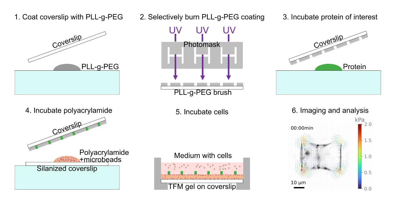
Figure 1. Schematic illustrating the procedure of a traction force microscopy (TFM) experiment on micropatterned samples
A. Coverslip silanization
This treatment ensures that the polyacrylamide gel will stick to the glass. All steps should be performed under a fume hood since bind silane is volatile and toxic.
1. Place as many coverslips as you can fit into the lid of a 145 mm Petri dish (because the lid can fit more coverslips than the base).
2. Pour 10 mL of silanization solution into the lid and cover with a second lid of a 145 mm Petri dish to avoid evaporation.
3. Incubate for at least 5 min.
4. Either dispose of the silanization into appropriate chemical waste or reuse it for a second batch of coverslips (prepared in another lid).
5. Rinse once or twice with 96% ethanol.
6. Remove coverslips while still covered with ethanol; otherwise, they will stick to the plastic. Take coverslips out with a tweezer and put them on a paper towel.
7. Dry carefully with another paper towel. Do not let the coverslips dry by themselves, as that will leave traces that could potentially be problematic for imaging.
8. Store silanized coverslips in a Petri dish for up to several months.
B. Clean coverslips for micropatterning
1. Clean coverslips with isopropanol and Kimwipes or use a coverslip rack, a beaker filled with isopropanol, and an ultrasonic bath to clean several coverslips at a time.
2. Use a nitrogen spray gun to dry the coverslips and remove dust.
3. Activate/clean the coverslips and the photomask in a plasma cleaner at 0.4 mbar with air atmosphere for 5 min.
C. Passivate coverslips with PLL-g-PEG
This step renders the coverslip anti-adhesive to both protein and cells. Subsequent removal of this passivation layer in specific places through photolithography allows for the patterning of the coverslip.
1. Put a drop of PLL-g-PEG solution on parafilm.
2. Take each coverslip with tweezers and flip it on the droplet with the plasma-activated side facing the PLL-g-PEG solution.
3. Let incubate for 30 min.
4. At the end of the incubation, lift the coverslips carefully without scratching the coating.
5. Clean the coverslips with a squirt bottle of MilliQ water. The PLL-g-PEG side should be very hydrophobic, and the water should go down easily.
6. Dry coverslips completely with a nitrogen spray gun or let them dry on a Kimwipe.
D. Deep UV burning and protein coating
This step removes the passivation layers from the previous step in specific places through photolithography, which allows for the patterning of the coverslip.
1. Make sure the photomask has been properly cleaned by the previous user (see section E).
2. Heat up the UV lamp for at least 5 min to reach a stable light intensity.
3. Rest the mask on a horizontal surface with the chrome side facing up.
4. Put a little drop of MilliQ water on the region of interest on the mask. Flip the coverslip onto the drop of water, with the PLL-g-PEG side facing the water. Remove excess water with a Kimwipe while applying pressure with your thumb. Wear gloves to not leave any traces on the mask or the coverslip. As much water as possible should be removed, so that there is good contact between the coverslip and the photomask. If good contact is established, you should see refraction patterns when looking at reflecting light on the coverslip.
5. Put the photomask in the warmed UV lamp with the coverslip-containing side facing away from the UV source. Place the photomask on three Petri dishes to avoid having the mask resting on the coverslips. Expose to UV light for 5 min.
6. Prepare the protein coating solution by diluting fibronectin to 20 μg/mL in 100 mM sodium bicarbonate.
7. After 5 min of UV light exposure, pour MilliQ water to help detach the coverslips from the mask. You can use a scalpel or tweezers (ideally with Teflon tips). When detaching the coverslips from the photomask, be very careful not to damage the mask. The patterned part of the coverslip is now hydrophilic, and the patterns can be seen when pouring water over the coverslip.
8. Put a drop of protein solution on parafilm (42 μL for 25 mm coverslips) and put the functionalized side of the coverslip on the droplet. Let it incubate for 30 min.
9. Pour MilliQ water over the coverslips, detach from the parafilm, and then rinse the coverslips with a squirt bottle of MilliQ water.
E. Mask cleaning
1. Wash the photomask with water and soap. Rub the surface gently with gloves.
2. Rinse the mask with plenty of deionized water and dry it with a nitrogen spray gun.
3. Rest the mask on a Kimwipe and pour isopropanol on it. Use another Kimwipe to thoroughly rub the surface of the mask.
4. Rinse the mask with 96% ethanol and dry it thoroughly with a nitrogen spray gun.
5. Put the mask in a plasma cleaner and pull a vacuum. Flush the chamber with oxygen for 5 min.
6. Pull a vacuum again and stabilize the pressure at 0.4 mbar. Activate the plasma for 10 min.
F. Polymerization and transfer of micropatterns to polyacrylamide gel
These steps should be performed quickly as polymerization starts as soon as APS is added, and if it proceeds too far before the micropatterned coverslip is placed, the drop might not spread completely. Once the acrylamide solution starts polymerizing, it is not toxic anymore and can be removed from the fume hood.
1. Mix 200 μL of polyacrylamide premix with 0.5 μL of FluoSpheres and vortex vigorously.
2. Put the premix in a vacuum chamber for 10 min to remove bubbles.
3. Ultrasonicate for 3 min.
4. Prepare a pipette with 42 μL and another with 1 μL.
5. Place silanized coverslips (functionalized surface facing up) on the top of a large Petri dish covered with parafilm.
6. Add 1 μL of TEMED and then 1 μL of APS and vortex vigorously.
7. Place a drop of 42 μL of the polyacrylamide solution onto the silanized coverslips and carefully place the micropatterned coverslip on top, with the patterned side facing the polyacrylamide solution.
8. Let the solution polymerize for 30 min.
9. Use the remaining acrylamide in the vial to check if polymerization was successful.
10. Pour deionized water over the polyacrylamide gels and let them hydrate for a few minutes.
11. Carefully detach the micropatterned coverslip with a scalpel. Do not force them apart, go carefully around the edges with the scalpel and allow the water to enter through the opening.
12. Place the coverslip in a 32 mm Petri dish or 6-well plate and rinse a few times with PBS until use.
G. Cell seeding
This protocol was used for cell seeding of MDCK cells expressing an optogenetic construct that allows activation of RhoA with the use of light. The specific parameters, such as incubation time for cell detachment, need to be adapted to the cell type.
1. Preheat cell detachment solution, sterile PBS, and cell culture medium to 37 °C in a water bath.
2. Put the coverslip with TFM gel in a coverslip cell chamber and rinse a few times with sterile PBS.
3. Add 1 mL of cell culture medium, put a lid from a Petri dish, and preheat in the incubator.
4. Remove the cell culture medium from the cell culture flask and rinse cells once or twice with sterile PBS to remove dead cells and cell debris.
5. Add cell detachment solution to cells. For a T25 cell culture flask, add 1 mL. Incubate for roughly 10–20 min. Frequent pipetting and tapping of the flask against the workbench helps to accelerate the process. Check frequently with a microscope the progress of cell detachment.
6. Transfer the cells in cell detachment solution to a 15 mL centrifugation tube and add 4 mL of cell culture medium.
7. Centrifuge at 234× g for 3 min to concentrate cells at the bottom of the tube.
8. Remove supernatant and resuspend in 5 mL of fresh cell culture medium.
9. Dilute part of the cell suspension to have the desired number of cells per sample in 1 mL of medium. Put some of the remaining cells back into cell culture.
10. To determine the number of cells to seed per sample, estimate the number of patterns on your coverslip and multiply by the number of cells per pattern. In our case, we had approximately 30,000 patterns, and we wanted to have one cell per pattern, so we seeded approximately 30,000 cells per sample.
11. Seed 1 mL of the correctly diluted cell suspension per sample. Pipetting tends to create liquid flow in the dish, which tends to concentrate cells in the center. To combat this and to get a more homogeneous seeding, pipette slowly while going in circles around the edge of the coverslip.
12. Incubate for 16–28 h to allow cells to divide on the patterns and form doublets or for 4–12 h to study single cells.
H. Imaging
We did all our imaging on a Nikon Ti-E2 microscope with an Orca Flash 4.0 sCMOS camera (Hamamatsu), a temperature control system set at 37 °C, a humidifier, and a CO2 controller, but any standard epifluorescence microscope can be used for TFM experiments. We strongly recommend the use of a drift correction system when acquiring movies, since small changes in focus can already strongly impact force measurements. We used and recommend physical drift correction systems, such as the PFS of Nikon, because of their speed and ease of use. If no microscope with such a system is available, drift correction systems based on real-time image analysis can be used, such as the drift correction software included in iTACS by Nguyen et al. [23]. Spinning disks or classical confocal microscopes can also be used. In this case, we recommend acquiring a small z-stack of a few micrometers around the top plane of the gel and averaging the images. If only one plane is taken, very small drifts, which usually happen even with drift correction systems, lead to images where the FluoSphere changes in size while going in and out of the focal plane, which can have an impact on the displacement measurements.
For the camera, a small pixel size is preferable over high sensitivity. The FluoSpheres in the gel are very bright, so high sensitivity is not necessary, and the pixel size is proportional to the resolution of displacement measurement. For the same reason, high magnifications (e.g., 60×) should be used when high precision is required. In principle, with particle tracking velocimetry, FluoSpheres movements can be measured with subpixel precision, but in practice, such a small signal would be indistinguishable from noise. On the other hand, too high displacements can lead to measurement errors. To get good displacement measurements, the rigidity of the gel should be chosen such that typical displacements fall between around 0.5 and 15 bead diameters (Figure 2).
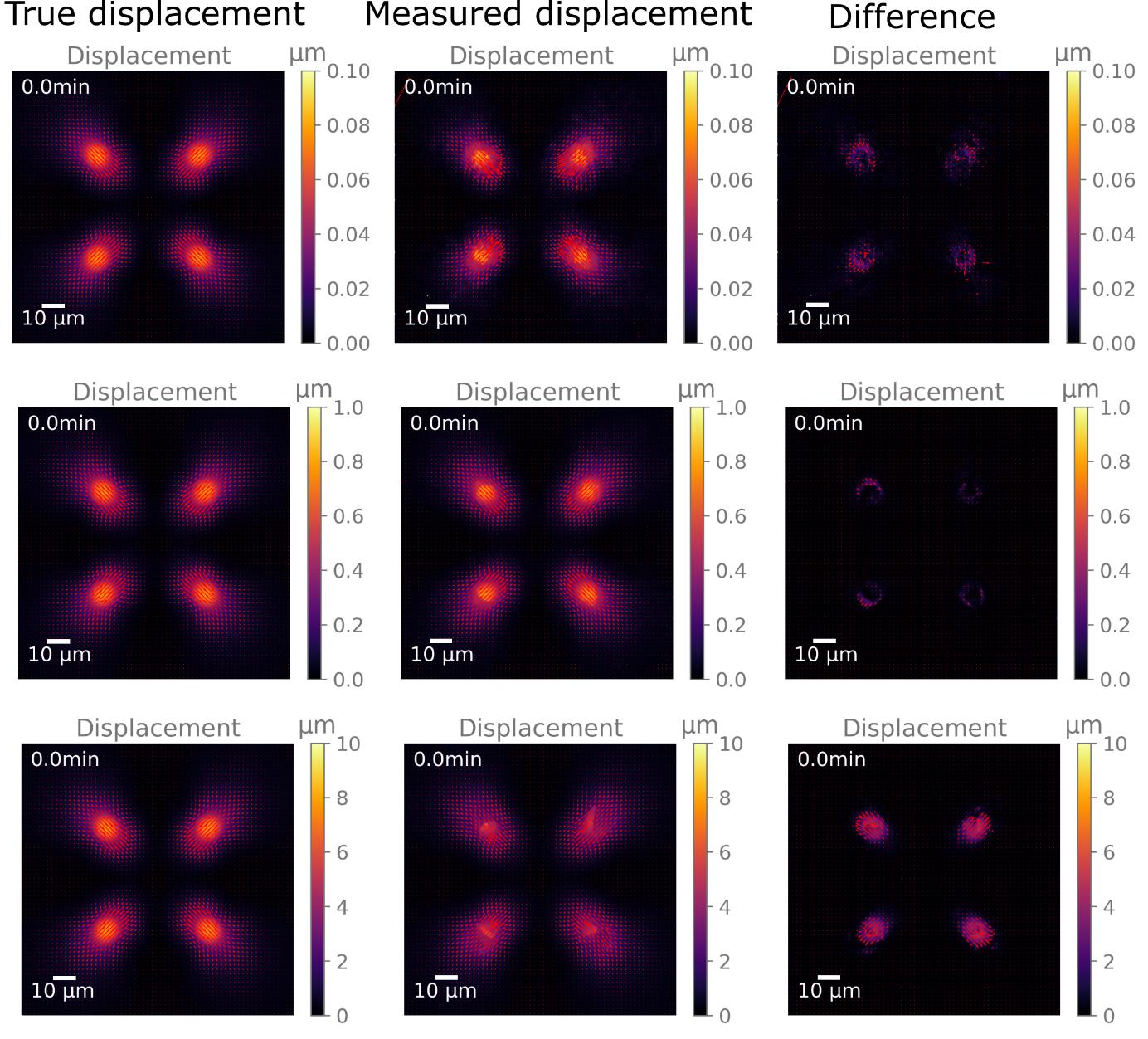
Figure 2. Illustration of the impact of displacement magnitude on measurement accuracy. The left column shows artificially generated displacement maps, which were used to deform an example bead image. The middle column shows the result of the displacement measurements between the deformed and original images. The right column shows the difference between the measured and true displacement. The top row contains data from small displacements, the middle row from medium, “ideal” displacements, and the bottom row from high displacements.
Data analysis
We process our data with custom-written Python code, which can be downloaded from https://github.com/ArturRuppel/batchTFM. Note that this is an updated version compared to the code that was used in our study that this protocol is based on [24]. The old version was written in MATLAB and is no longer maintained by the author. The most important change is the switch from Particle Image Velocimetry + Particle Tracking Velocimetry to optical flow for the gel deformation measurement. We have compared the two versions and found no significant difference (see protocol validation).
First, create one folder for each position called “position”+index (i.e., “position0” for the first position and “position1” for the second one, as seen in the “test_data” folder on https://github.com/ArturRuppel/batchTFM). These folders need to contain a stack of images of the fluorescent beads while cells are attached to the hydrogel and one image of the beads after the removal of the cells when the hydrogel is in the relaxed state. At least one and up to three stacks of images of the cells need to be added as well. These images do not impact the data analysis; the code only corrects for translation through image registration. This allows to couple precise cell morphology and/or protein localization measurements with force localization. In the end, the script produces a movie of the first stack with the forces overlaid.
Analysis parameters
All data analysis parameters are found in the file “main.py” (Figure 3). First, set them according to your experiment and then run the script in your Python IDE (e.g., spyder).
The “path” parameter is a string, which should contain the path to the folder “position + index”. The different “name” parameters should contain a string with the filename of your images. We usually call “AK” (After Kill) the image of the beads in the relaxed state, “BK” (Before Kill) the movies of the beads in the stressed state, and “fluo” the image stack of the cells.
The “no_stacks” parameter represents the number of positions you want to analyze. “finterval” represents the time interval between two frames in minutes, “pixelsize” represents the physical size of a pixel in the bead images in micrometers, and “downsamplerate” represents the factor by which the final displacement and force maps are downsized. This serves mainly to conserve disk space. If set at 1, the displacement and force maps will have the same size as the bead images.
Then, choose which part of the analysis you want to launch on your data by uncommenting lines calling said functions (Figure 4). If one or several parts of the analysis are already done, they can be skipped by adding a “#” in front of the corresponding function.
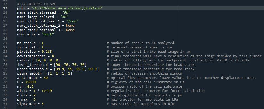
Figure 3. Screenshot extracted from “main.py” that shows the parameters to set before running the code
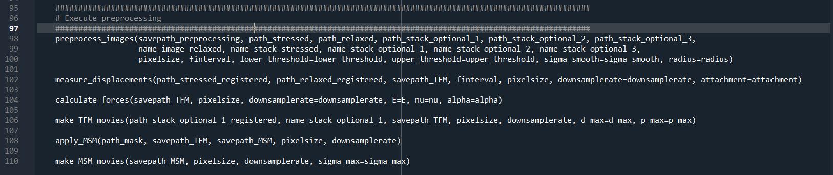
Figure 4. Screenshot extracted from “main.py” showing the part where the steps to perform can be selected or unselected. Depending on which functions are enabled, more parameters need to be set in the “parameters to set” part of “main.py” (Figure 3).
The “preprocess_images” function takes all images described before and returns images with an adjusted contrast. Additionally, it aligns all bead images to the bead image in the relaxed state to correct translational xy drift from the microscope stage. It also applies the same translations to the additional cell images. This ensures that all images are well aligned at all time points, which is crucial if measurements on the cell images need to be combined with the TFM data. The outputs of this function are the processed image files, stored in a folder called “preprocessed_images” in the folder of the corresponding position.
The parameters “lower_threshold” and “upper_threshold” represent the percentile values for the contrast adjustment. The four different numbers correspond to the four different image stacks that can be put in. The first one corresponds to the bead images and the subsequent one for the cell images. The threshold values are the same for all the beads images, both in the relaxed and stressed state, so make sure that they were all acquired with the same imaging parameters.
The parameter “sigma_smooth” describes the size of the Gaussian kernel in pixels with which the images are smoothened. The “radius” variable corresponds to the size of a ball used for the “rolling ball background subtraction” algorithm (see doc skimage: https://scikit-image.org/docs/stable/auto_examples/segmentation/plot_rolling_ball.html). Smoothening and background subtraction are usually not necessary if images have a decent contrast and are likely to influence the measurement results. To skip these, set the radius to 0 and the smoothening window to 1. These features can still be useful if one wishes to qualitatively analyze failed experiments, or if acquiring high-contrast images is not possible. This part of the code returns a processed version of the user’s images and stacks in a folder called “preprocessed images.”
The “measure_displacement” function takes the images of the preprocessed images of the beads and returns the displacement matrices of the soft gel along the x- and y-axis. The output files are called “d_x.npy” and “d_y.npy” and are saved in the TFM_data folder created automatically in the “position+index” folder. These displacement matrices are obtained from estimations of the optical flow between each frame of the stressed bead images and the relaxed bead image. This function uses “optical_flow_tvl1” [26–28], a variational method that allows to compute an estimation of the optical flow between the bead images and returns the estimated displacement of the soft gel upon stress applied by the cells. The matrices returned by this function will be the size of the images of the beads divided by the “downsamplerate” defined earlier. (For example, if the size of the bead images is 600 × 600 pixels and the downsamplerate is 4, then the displacement matrix will be 150 × 150 pixels.) Each element of these matrices represents a pixel of the displacement map, and each pixel is associated with an estimation of the displacement of the soft gel quantified in micrometers along the x-axis for “d_x.npy” or the y-axis for “d_y.npy.”
The “calculate_forces” function solves the inverse problem to compute an estimation of the traction forces that were applied by the cells on the soft gel to observe the estimated displacements measured by the preceding function. It uses the classical approach of transforming the displacement field into the Fourier space to solve the corresponding equations. This approach is called Fourier Transform Traction Cytometry (FTTC) and was initially proposed by Butler et al. [11]. Before launching this function, define the Young modulus (called “E”) and the Poisson ratio (called “nu”) of the hydrogel used for the experiment you want to analyze. For example, in the associated paper from Ruppel et al. [24], a gel of approximately 19.66 kPa was used, so E = 19660. This gel is made of polyacrylamide, which has a Poisson ratio of 0.5. The traction forces are calculated via the solution of a linear system and from under-sampled data with potential acquisition noise. To correct for this, the function uses a regularization scheme, which effectively smoothens the output in the disfavor of overfitting the force field to a noisy displacement field. The regularization parameter is called “alpha” in the code, and we usually determine it empirically by setting it as low as possible without getting too much noise in the force fields. See Sabass et al. for a more detailed discussion of regularization in TFM calculations [29]. This function returns two matrices of the traction forces along the x- and y-axis defined arbitrarily by the horizontal and vertical axes of the images. These matrices have the same dimensions as the displacement matrices described earlier. Each element of these matrices is a spatial region associated with a value of the traction forces. As we have two matrices and two axes along which the tractions are applied, we can reconstruct a traction vector and represent the amplitude and the orientation of the forces applied by the cells on the substrate in a 2D traction force map.
The function "make_TFM_movies" is used to create movies or images of the traction force maps and to generate displacement maps. These maps represent the displacements of the gel under the cells using vectors, where the length and color indicate the magnitude of the displacement, and the orientation shows the direction of the bead displacement. The function also allows the user to get a version of the traction force map assembled with a potential brightfield or fluorescent channel to allow them to have a first impression of the link between the mechanical readouts calculated with the TFM and the morphology of the cells.
The function “apply_MSM” is used to perform monolayer stress microscopy, which takes the TFM data computed earlier and a mask with the contour of the cell layer to compute the internal mechanical stresses of the cell layer. It uses the MSM functions developed by the Fabry Lab, which can be found in the free Python package pyTFM [2]. MSM models the cell layer as a thin plate with linear and homogeneous material properties and then solves the associated partial differential equations to obtain internal mechanical stresses from the traction force data. For a detailed discussion of this method, see Tambe et al. [15]. The function “apply_MSM” returns a matrix that contains the Cauchy stress tensor for each pixel and each frame of the initial traction force image. The main diagonals of this stress tensor are the normal stresses in x- and in y-direction, respectively, and the off-diagonals correspond to the shear stresses.
Similar to “make_TFM_movies,” the “make_MSM_movies” function allows the user to generate movies that represent spatially the evolution of the internal stresses of the system from the MSM data. The function generates a movie for the two normal stresses along the x- and y-axes and also a global representation of the average normal stress in the system.
Validation of protocol
We validated the accuracy of our TFM code by analyzing a synthetic dataset. For this, we used code from Blumberg et al. [30] to generate an example displacement and traction force field that looks similar to what we typically observed in our experiments. Then, we applied this deformation field to an example bead image from one of our experiments. Finally, we used both the no longer supported MATLAB code and the new “batchTFM” code to find the deformation map between these two images. The results are shown in Figure 5. The main difference between these two versions of the script is the method used to find these deformation maps. The MATLAB code uses a combination of particle image velocimetry (PIV) combined with particle tracking velocimetry (PTV) to find this deformation map, and batchTFM uses an optical flow algorithm to find the same deformation map. As seen in Figure 5, the deformation maps obtained from these two methods are virtually identical. Figure 5 also shows the traction force maps calculated from the deformation maps. The same Fourier transform traction cytometry (FTTC) algorithm was used in both cases. In both cases, the original traction force maps are reproduced faithfully, albeit with some background force level and an underestimation of the peak force value. This is unavoidable and a direct consequence of the ill-posed nature of the force reconstruction problem and the hence necessary regularization scheme described earlier. To illustrate the output of the algorithm, Figure 6 shows force maps comparing cell doublets with single cells on H-shaped micropatterns.
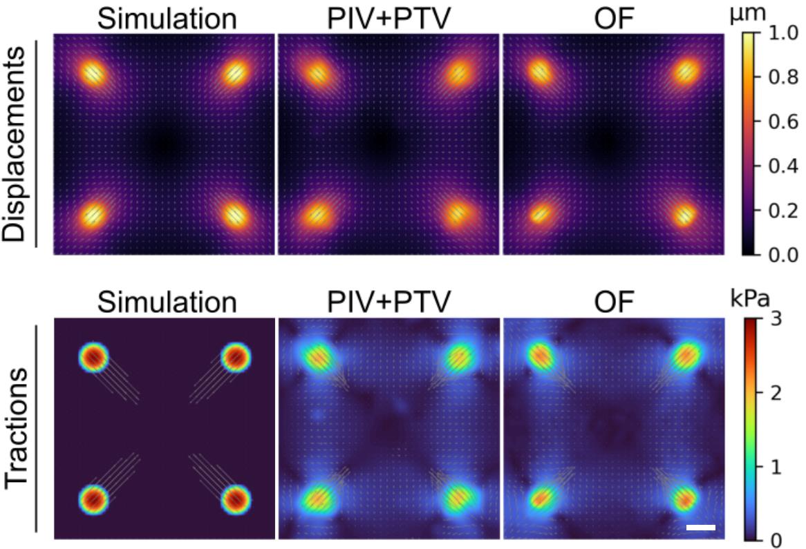
Figure 5. The simulated displacement field on the top left was used to deform an example image of beads and these two images were then used to test the two different displacement measurement methods, namely particle image velocimetry (PIV) combined with particle tracking velocimetry (PTV) compared with optical flow (OF). The bottom row shows the correct traction stress field for the simulated data on the left. Taken from [31]. Scale bar is 10 μm.
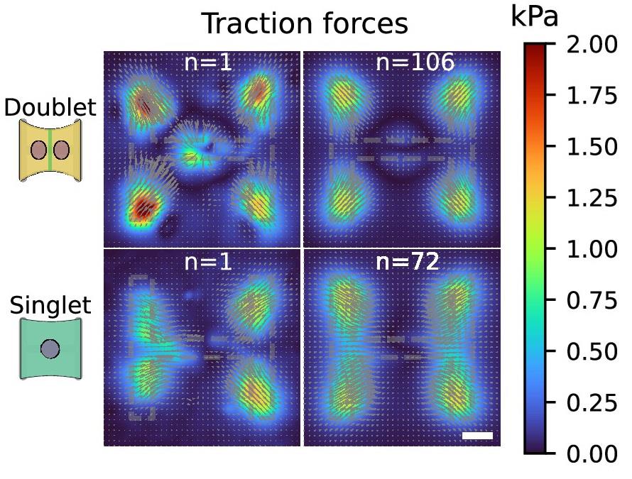
Figure 6. Example of traction force data, comparing an example and the average traction of cell doublets and single cells on H-shaped micropatterns. Taken from [24]. Scale bar is 10 μm.
The MSM part of the analysis, which is part of the pyTFM software, has been validated by the developers of the software in [2].
General notes and troubleshooting
General notes
Setting up TFM experiments can be challenging; specifically, the analysis and interpretation of the data can become very technical. Once everything is set up, however, it works very reliably and can be used routinely. Do not hesitate to reach out if you need help setting up your TFM experiments.
Troubleshooting
Problem 1: The polyacrylamide gel does not polymerize properly.
Possible cause: The APS is not active anymore. APS is unstable in water and the powder tends to absorb water from the air.
Solution: Use fresh APS.
Problem 2: The micropatterns do not transfer well to the gel.
Possible cause: This usually happens only with micropatterns that have a big surface area (approximately >10.000 µm2).
Solution: Unfortunately, there is no simple solution to the problem. For big patterns, we recommend adding a crosslinker to the gel or using microcontact printing instead. Please contact us for more details if you have this issue.
Problem 3: The beads cluster under the micropattern.
Possible cause: This happens almost always and is due to unspecific interactions between your protein of interest and the beads.
Solution: We do not think that this is a problem as long as there are still enough beads in the immediate vicinity of the pattern. Outside of the pattern, the gel does not deform because there are no cells, so it is not a problem if there are fewer beads there.
Problem 4: There are a lot of displacement vectors at the edges of the image but there are no cells.
Possible cause: This is due to spherical aberrations at the edges of the image. This problem is exacerbated with cameras that have a large field of view.
Solution: Place your cells in the center of the image and crop the borders.
Problem 5: The displacement field is completely nonsensical, e.g., there is a rotational field in the whole field of view.
Possible cause: When trypsinizing the cells to take the reference images, it is extremely important to move the sample as little as possible. Small, translational drift is compensated by the algorithm, but large displacements or rotational movements will lead to nonsensical results or to an error message. Sometimes, the data can still be saved through additional image registration and/or manual alignment.
Solution: Do not touch the sample when trypsinizing the cells.
Problem 6: The resulting displacement field is extremely noisy.
Possible cause: The background in the bead image was not removed properly.
Solution: Either the contrast of the bead images is too low, or the threshold value in the algorithm is too low. In the former case, the experiment should be redone with higher light intensity and/or exposure time; in the latter case, only the threshold value in the algorithm needs to be adjusted.
Problem 7: The resulting displacement field is extremely noisy.
Possible cause: The forces generated by the cells are very weak.
Solution: Some cell types exert very little to no force. These can be very challenging to measure. Using softer gels can help, but typically this will also increase the noise. In any case, the smaller the forces one tries to measure, the more important it is to get good contrast and resolution in the imaging data.
Acknowledgments
This protocol describes the experiments done in our original study published in eLife [24]. We acknowledge the use of GPT 3.5 for generating a first draft of the Procedure section. We acknowledge the Agence Nationale de la Recherche (ANR-17-CE30-0032-01) for funding. Most importantly, we would like to thank Andreas Bauer and Ben Fabry for publishing pyTFM, which was crucial to accomplishing the study this protocol refers to.
Competing interests
There is no conflict of interest we are aware of.
References
- Tseng, Q., Wang, I., Duchemin-Pelletier, E., Azioune, A., Carpi, N., Gao, J., Filhol, O., Piel, M., Théry, M., Balland, M., et al. (2011). A new micropatterning method of soft substrates reveals that different tumorigenic signals can promote or reduce cell contraction levels. Lab Chip. 11(13): 2231. https://doi.org/10.1039/c0lc00641f
- Bauer, A., Prechová, M., Fischer, L., Thievessen, I., Gregor, M. and Fabry, B. (2021). pyTFM: A tool for traction force and monolayer stress microscopy. PLoS Comput Biol. 17(6): e1008364. https://doi.org/10.1371/journal.pcbi.1008364
- Chen, C. S., Mrksich, M., Huang, S., Whitesides, G. M. and Ingber, D. E. (1997). Geometric Control of Cell Life and Death. Science. 276(5317): 1425–1428. https://doi.org/10.1126/science.276.5317.1425
- McBeath, R., Pirone, D. M., Nelson, C. M., Bhadriraju, K. and Chen, C. S. (2004). Cell Shape, Cytoskeletal Tension, and RhoA Regulate Stem Cell Lineage Commitment. Dev Cell. 6(4): 483–495. https://doi.org/10.1016/s1534-5807(04)00075-9
- Tseng, Q., Duchemin-Pelletier, E., Deshiere, A., Balland, M., Guillou, H., Filhol, O. and Théry, M. (2012). Spatial organization of the extracellular matrix regulates cell–cell junction positioning. Proc Natl Acad Sci USA. 109(5): 1506–1511. https://doi.org/10.1073/pnas.1106377109
- Wang, N., Ostuni, E., Whitesides, G. M. and Ingber, D. E. (2002). Micropatterning tractional forces in living cells. Cell Motil. 52(2): 97–106. https://doi.org/10.1002/cm.10037
- Harris, A. K., Wild, P. and Stopak, D. (1980). Silicone Rubber Substrata: A New Wrinkle in the Study of Cell Locomotion. Science. 208(4440): 177–179. https://doi.org/10.1126/science.6987736
- Lee, J., Leonard, M., Oliver, T., Ishihara, A. and Jacobson, K. (1994). Traction forces generated by locomoting keratocytes. J Cell Biol. 127(6): 1957–1964. https://doi.org/10.1083/jcb.127.6.1957
- Pelham, R. J. and Wang, Y. l. (1999). High Resolution Detection of Mechanical Forces Exerted by Locomoting Fibroblasts on the Substrate. Mol Biol Cell. 10(4): 935–945. https://doi.org/10.1091/mbc.10.4.935
- Dembo, M., Oliver, T., Ishihara, A. and Jacobson, K. (1996). Imaging the traction stresses exerted by locomoting cells with the elastic substratum method. Biophys J. 70(4): 2008–2022. https://doi.org/10.1016/s0006-3495(96)79767-9
- Butler, J. P., Tolić-Nørrelykke, I. M., Fabry, B. and Fredberg, J. J. (2002). Traction fields, moments, and strain energy that cells exert on their surroundings. Am J Physiol, Cell Physiol. 282(3): C595–C605. https://doi.org/10.1152/ajpcell.00270.2001
- Schwarz, U. S. and Soiné, J. R. (2015). Traction force microscopy on soft elastic substrates: A guide to recent computational advances. Biochim Biophys Acta Mol Cell Res. 1853(11): 3095–3104. https://doi.org/10.1016/j.bbamcr.2015.05.028
- Maruthamuthu, V., Sabass, B., Schwarz, U. S. and Gardel, M. L. (2011). Cell-ECM traction force modulates endogenous tension at cell–cell contacts. Proc Natl Acad Sci USA. 108(12): 4708–4713. https://doi.org/10.1073/pnas.1011123108
- Liu, Z., Tan, J. L., Cohen, D. M., Yang, M. T., Sniadecki, N. J., Ruiz, S. A., Nelson, C. M. and Chen, C. S. (2010). Mechanical tugging force regulates the size of cell–cell junctions. Proc Natl Acad Sci USA. 107(22): 9944–9949. https://doi.org/10.1073/pnas.0914547107
- Tambe, D. T., Corey Hardin, C., Angelini, T. E., Rajendran, K., Park, C. Y., Serra-Picamal, X., Zhou, E. H., Zaman, M. H., Butler, J. P., Weitz, D. A., et al. (2011). Collective cell guidance by cooperative intercellular forces. Nat Mater. 10(6): 469–475. https://doi.org/10.1038/nmat3025
- Tambe, D. T., Croutelle, U., Trepat, X., Park, C. Y., Kim, J. H., Millet, E., Butler, J. P. and Fredberg, J. J. (2013). Monolayer Stress Microscopy: Limitations, Artifacts, and Accuracy of Recovered Intercellular Stresses. PLoS One. 8(2): e55172. https://doi.org/10.1371/journal.pone.005517
- Nier, V., Jain, S., Lim, C. T., Ishihara, S., Ladoux, B. and Marcq, P. (2016). Inference of Internal Stress in a Cell Monolayer. Biophys J. 110(7): 1625–1635. https://doi.org/10.1016/j.bpj.2016.03.002
- Ng, M. R., Besser, A., Brugge, J. S. and Danuser, G. (2014). Mapping the dynamics of force transduction at cell–cell junctions of epithelial clusters. eLife. 3: e03282. https://doi.org/10.7554/elife.03282
- Lendenmann, T., Schneider, T., Dumas, J., Tarini, M., Giampietro, C., Bajpai, A., Chen, W., Gerber, J., Poulikakos, D., Ferrari, A., et al. (2019). Cellogram: On-the-Fly Traction Force Microscopy. Nano Lett. 19(10): 6742–6750 https://doi.org/10.1021/acs.nanolett.9b01505
- Barrasa-Fano, J., Shapeti, A., Jorge-Peñas, Ã., Barzegari, M., Sanz-Herrera, J. A. and Van Oosterwyck, H. (2021). TFMLAB: A MATLAB toolbox for 4D traction force microscopy. SoftwareX. 15: 100723. https://doi.org/10.1016/j.softx.2021.100723
- Mittal, N. and Han, S. J. (2021). High‐Resolution, Highly‐Integrated Traction Force Microscopy Software. Curr Protocol. 1(9): e233. https://doi.org/10.1002/cpz1.233
- Carl, P. and Rondé, P. (2023). JEasyTFM: an open-source software package for the analysis of large 2D TFM data within ImageJ. Bioinf Adv. 3(1): e1093/bioadv/vbad156. https://doi.org/10.1093/bioadv/vbad156
- Nguyen, A., Battle, K., Paudel, S. S., Xu, N., Bell, J., Ayers, L., Chapman, C., Singh, A. P., Palanki, S., Rich, T., et al. (2022). Integrative Toolkit to Analyze Cellular Signals: Forces, Motion, Morphology, and Fluorescence. J Visualized Exp. 181: e3791/63095. https://doi.org/10.3791/63095
- Ruppel, A., Wörthmüller, D., Misiak, V., Kelkar, M., Wang, I., Moreau, P., Méry, A., Révilloud, J., Charras, G., Cappello, G., et al. (2023). Force propagation between epithelial cells depends on active coupling and mechano-structural polarization. eLife. 12: e83588. https://doi.org/10.7554/elife.83588
- Tse, J. R. and Engler, A. J. (2010). Preparation of Hydrogel Substrates with Tunable Mechanical Properties. Curr Protoc Cell Biol. 47(1): ecb1016s47. https://doi.org/10.1002/0471143030.cb1016s47
- Zach, C., Pock, T. and Bischof, H. (2007). A Duality Based Approach for Realtime TV-L 1 Optical Flow. Lect Notes Comput Sci. 214–223. https://doi.org/10.1007/978-3-540-74936-3_22
- Wedel, A., Pock, T., Zach, C., Bischof, H. and Cremers, D. (2009). An Improved Algorithm for TV-L 1 Optical Flow. Lect Notes Comput Sci. : 23–45. https://doi.org/10.1007/978-3-642-03061-1_2
- Sánchez Pérez, J., Meinhardt-Llopis, E. and Facciolo, G. (2013). TV-L1 Optical Flow Estimation. Image Processing On Line 3: 137–150. https://doi.org/10.5201/ipol.2013.26
- Sabass, B., Gardel, M. L., Waterman, C. M. and Schwarz, U. S. (2008). High Resolution Traction Force Microscopy Based on Experimental and Computational Advances. Biophys J. 94(1): 207–220. https://doi.org/10.1529/biophysj.107.113670
- Blumberg, J. W. and Schwarz, U. S. (2022). Comparison of direct and inverse methods for 2.5D traction force microscopy. PLoS One. 17(1): e0262773. https://doi.org/10.1371/journal.pone.0262773
- Ruppel, A. (2022). Optogenetic interrogation of intercellular propagation of force signals. PhD Thesis.
文章信息
稿件历史记录
提交日期: Jun 3, 2024
接收日期: Oct 29, 2024
在线发布日期: Nov 21, 2024
出版日期: Jan 5, 2025
版权信息
© 2025 The Author(s); This is an open access article under the CC BY license (https://creativecommons.org/licenses/by/4.0/).
如何引用
Readers should cite both the Bio-protocol article and the original research article where this protocol was used:
- Ruppel, A., Misiak, V. and Balland, M. (2025). An Open-source Python Tool for Traction Force Microscopy on Micropatterned Substrates. Bio-protocol 15(1): e5156. DOI: 10.21769/BioProtoc.5156.
- Ruppel, A., Wörthmüller, D., Misiak, V., Kelkar, M., Wang, I., Moreau, P., Méry, A., Révilloud, J., Charras, G., Cappello, G., et al. (2023). Force propagation between epithelial cells depends on active coupling and mechano-structural polarization. eLife. 12: e83588. https://doi.org/10.7554/elife.83588
分类
生物信息学与计算生物学
生物物理学 >
细胞生物学 > 基于细胞的分析方法
您对这篇实验方法有问题吗?
在此处发布您的问题,我们将邀请本文作者来回答。同时,我们会将您的问题发布到Bio-protocol Exchange,以便寻求社区成员的帮助。