

Fluorescence-based Single-cell Analysis of Whole-mount-stained and Cleared Microtissues and Organoids for High Throughput Screening
基于荧光的全染色单细胞分析和清除的微组织和类器官高通量筛选
发布: 2021年06月20日第11卷第12期 DOI: 10.21769/BioProtoc.4050 浏览次数: 5866
评审: Ralph Thomas BoettcherTalita Diniz Melo HanchukDana Manuela SavulescuOlga Kopach
参见作者原研究论文
The authors used this protocol in:

Nov 2020
Advertisement


Abstract
Three-dimensional (3D) cell culture, especially in the form of organ-like microtissues (“organoids”), has emerged as a novel tool potentially mimicking human tissue biology more closely than standard two-dimensional culture. Typically, tissue sectioning is the standard method for immunohistochemical analysis. However, it removes cells from their native niche and can result in the loss of 3D context during analyses. Automated workflows require parallel processing and analysis of hundreds to thousands of samples, and sectioning is mechanically complex, time-intensive, and thus less suited for automated workflows. Here, we present a simple protocol for combined whole-mount immunostaining, tissue-clearing, and optical analysis of large-scale (approx. 1 mm) 3D tissues with single-cell level resolution. While the protocol can be performed manually, it was specifically designed to be compatible with high-throughput applications and automated liquid handling systems. This approach is freely scalable and allows parallel automated processing of large sample numbers in standard labware. We have successfully applied the protocol to human mid- and forebrain organoids, but, in principle, the workflow is suitable for a variety of 3D tissue samples to facilitate the phenotypic discovery of cellular behaviors in 3D cell culture-based high-throughput screens.
Graphic abstract:
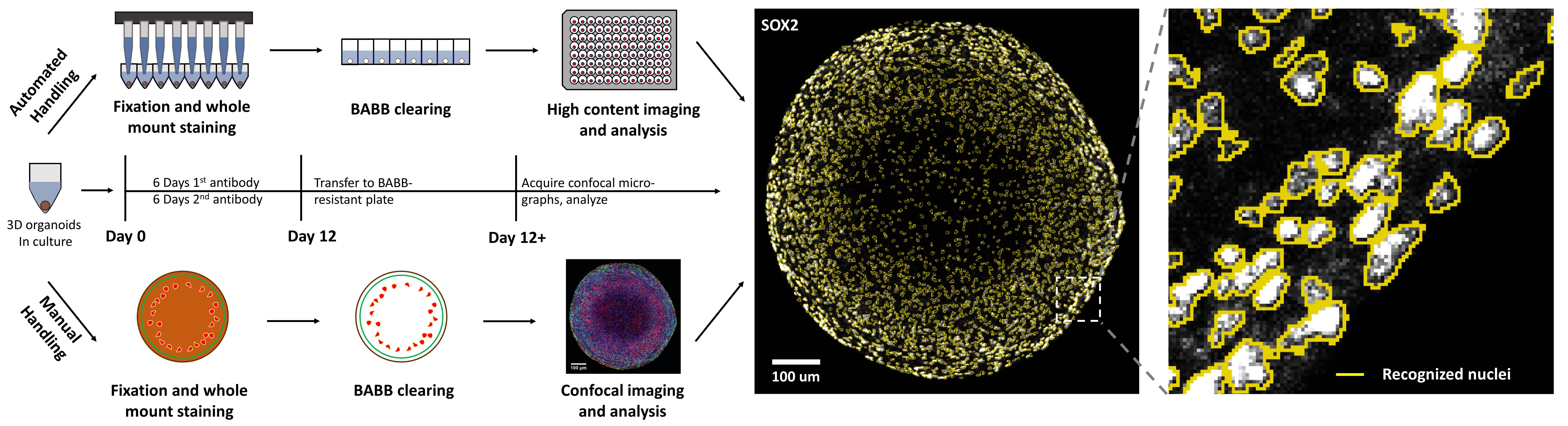
Automatable organoid clearing and high-content analysis workflow and timeline
Background
Over the past years, three-dimensional (3D) cell culture systems, in particular stem cell-based organoids, have enabled novel insights into human biology and disease (reviewed by: Rossi et al., 2018; Schutgens and Clevers, 2020; Kim et al., 2020). However, working with 3D models requires more than new cell culture techniques. Quantifying cells in complex 3D tissues in fast, unbiased, and efficient workflows requires adapting the analyses as well. So far, many studies have relied on tissue sectioning followed by immunostaining to analyze the structures and composition of their 3D aggregates in detail (Lancaster et al., 2013; Pasca et al., 2015). While this method has been invaluable, it requires ample manual intervention, is time-intensive and cumbersome, and thus not ideally suited for large-scale screening applications, including drug development campaigns. Moreover, sectioning provides only a view at a subset of sample tissue, often results in a loss of spatial information unless meticulous serial sections are prepared, and is challenging to use as a basis for 3D reconstruction.
More recently, the combination of whole-mount staining and tissue clearing allowed the analysis of entire 3D aggregates without the need for sectioning, as demonstrated by our group and others (Masselink et al., 2019; Dekkers et al., 2019; Renner et al., 2020). This approach allows rapid 3D acquisition of complex samples and preserves tissue context while providing single-cell-specific phenotypic information. Our workflow utilizes a customized immunostaining procedure, which we adapted and optimized for organoids based on a previous protocol (Lee et al., 2016). We combined this with benzyl alcohol benzyl benzoate (BABB)-based clearing (Dent et al., 1989), which clears human neural tissues quickly (minutes) and effectively (Renner et al., 2020). We specifically designed this procedure to be compatible with both manual pipetting and automated liquid handling systems, facilitating low- and high-throughput applications. Depending on the individual requirements, the samples can then be analyzed using a standard confocal microscope or a high-content imaging system. In either case, the resulting optical tissue cross sections enable the quantitative analysis of entire 3D samples down to the single-cell level. This eliminates the need to freeze/section the organoids and enables parallel staining and analysis of many samples in 96- or 384-well formats. Though we developed the workflow for the analysis of neural organoids, it is not restricted to a particular organoid system or sample type but can be applied to any 3D sample of interest.
Materials and Reagents
96-well plates, NuncTM MicroWellTM conical 96-well plates (V-bottom) (Thermo Fisher, catalog number: 277143)
Screenstar microplate, 96-well, COC, F-bottom, black (Greiner, catalog number: 655866)
Screw cap tubes (Sarstedt, catalog numbers: 62.547.254 [50 ml] and 62.554.502 [15 ml])
Serological pipets (Falcon, catalog numbers: 356543 [5 ml], 356551 [10 ml], and 356525 [25 ml])
Pipet tips (StarLab, catalog numbers: S1120-1810 [20 μl], S1120-8810 [200 μl], and S1122-1830 [1,000 μl])
Conical/V-bottom 96-well plates (Thermo Fisher, catalog number: 277143)
Optional: Biomek liquid handler pipette tips AP96 P250 (Beckman Coulter, catalog number: 717252)
Organoids/3D samples to be stained
Dulbecco's Phosphate Buffered Saline (PBS; Sigma-Aldrich, catalog number: D8662)
Paraformaldehyde (PFA; VWR, catalog number: 15714-S)
Triton X-100 (Roth, catalog number: 3051.2)
Sodium azide (Sigma-Aldrich, catalog number: 71289)
Bovine Serum Albumin (BSA, Thermo Fisher, catalog number: 15260037)
Methanol (Roth, catalog number: 4627.6)
Benzyl alcohol (Sigma-Aldrich, catalog number: 305197-100ML)
Benzyl benzoate (Sigma-Aldrich, catalog number: B6630-250ML)
Optional: Nuclear counterstain, e.g., DAPI (Sigma-Aldrich, catalog number: D9542-10MG)
Primary antibodies, depending on application [here: Rabbit anti-Tyrosine Hydroxylase (Abcam, product no: ab112) and Goat anti-Sox2 (R&D Systems, catalog number: AF2018)]
Secondary antibodies, depending on application [here: Donkey anti-Rabbit IgG, Alexa Fluor 647 (Thermo Fisher, catalog number: A-31573) and Donkey anti-Goat IgG, Alexa Fluor 568 (Thermo Fisher, catalog number: A-11057)]
Permeabilization buffer (see Recipes, Table 1)
Blocking solution (see Recipes, Table 2)
BABB/methanol (see Recipes, Table 3)
BABB (see Recipes, Table 4)
Equipment
Humidified CO2 incubator
Fridges and freezers (4°C, -20°C, and -80°C)
Optional: Stereomicroscope with camera (e.g., Leica MZ10 F (microscope) and Leica DFC425 C (camera), Leica Microsystems)
Mechanical pipettes
Optional: Multichannel mechanical pipettes
Optional: Automated liquid handling system (e.g., Biomek FXP Laboratory Automation Workstation, Beckman Coulter)
Confocal microscope (e.g., LSM 700, Zeiss)
Optional: High-content imaging system (e.g., Operetta high-content imager, Perkin Elmer)
Software
Fiji/ImageJ (Schindelin et al., 2012)
Optional: Leica application suite v 4.8 (LAS, Leica Microsystems)
Optional: Biomek Software v3.3 (controlling the automated liquid handler, Beckman Coulter)
Optional: High-content imaging and analysis software (e.g., Harmony v4.1, Perkin Elmer)
Optional: Excel (Microsoft Corporation)
Procedure
Caution: This protocol uses hazardous substances, including PFA, Triton X-100, methanol, benzyl alcohol, and benzyl benzoate. Be aware of toxicity from multiple routes of exposure, including inhalation. Refer to MSDS information before starting the procedure and work under a fume hood.
Note: All volumes mentioned here and in the following steps are optimized for samples in 96-well plates; other culture formats may require different volumes. For our setup and tissues with ca. 1 mm diameter or smaller, we use 150 μl of reagent volume per well. Larger volumes are possible and may be required for larger samples; however, we do not recommend going below 150 μl per well for fixation and washing to avoid having an insufficient amount of reagent for each tissue. For washing steps, higher volumes can increase the washing efficiency, but we found 150 μl per well to give good results.
Fixation of large-scale (approx. 1 mm) 3D tissues
Note: All steps described here can be performed either manually or using an automated liquid handling system (ALHS)/pipetting robot.
To fix the samples, carefully aspirate the media and add 150 μl of freshly prepared 4% PFA in PBS per well. Incubate for 10-15 min at room temperature.
Aspirate the fixative carefully and wash 3 × 5 min with 150 μl PBS per well.
Either add 150 μl PBS per well and seal the plate with parafilm to store the samples at 4°C or directly proceed with the staining procedure below.
Note: In our hands, several months of storage did not negatively impact the quality of the samples for whole-mount staining. However, we generally recommend quick turnaround times over longer storage.
Whole-mount immunostaining
Day 0Optional: Aspirate PBS carefully, add 150 µl of permeabilization buffer (see Recipes, Table 1) and incubate 1 h at 37°C.
Note: A dedicated permeabilization step is not generally required but may improve the outcome for specific markers/sample types. This must be optimized on a case-to-case basis.
Aspirate the permeabilization buffer/PBS and add 150 µl of primary antibody diluted in blocking solution (see Recipes, Table 2). Use antibody at the appropriate concentration (each antibody must be titrated and validated individually). Incubate 6 days at 37°C and 100% humidity, renewing the solution every 2nd day.
Notes on incubation times and conditions: 1. Incubation times depend on tissue size and density and the antibodies used. We recommend a prior optimization of the incubation times with representative test samples; this will save valuable time for follow-up experiments and assure optimum outcomes. We found 6 days of incubation per antibody to work well in our samples. 2. For the antibody incubation steps, do not seal the plates with parafilm as it may “melt” and become difficult to remove from the plate after longer incubation periods at 37°C. Incubators should be humidified to prevent evaporative loss of fluids in the plates (almost all tissue culture incubators work well for this step). 3. In our hands, samples did not show any signs of deterioration over this period. If necessary, 0.1% (w/v) sodium azide in blocking and staining solutions can prevent microbial growth during this time (see Recipes).
Note on control samples: Carefully plan control samples to be incubated without primary antibody to gauge non-specific binding of secondary antibody. Additionally, prepare control samples without antibodies to identify potential artifacts caused by autofluorescence. Quantitative assessment needs measurements of both types of background fluorescence to determine proper object-based detection thresholds for each channel.
Day 2
Renew primary antibody solution.
Renew primary antibody solution.
Wash samples with 150 μl 0.1% (v/v) Triton X-100 in PBS for 5 h at room temperature. Renew washing solution every hour.
Note: In case of issues with non-specific/high background signal, washing might be extended overnight and performed at 37°C.
Aspirate the washing solution carefully and add 150 µl of new blocking solution with secondary antibody 1:1,000 and DAPI (0.5 μg/ml). Incubate for 6 days at 37°C and 100% humidity. Renew solution every 2 days.
Note: This and all following incubation steps should be performed in the dark to preserve the fluorescence signals. We have extensively optimized the conditions for various AlexaFluor-conjugated secondary antibodies and always arrived at a 1:1,000 dilution. We have not optimized the conditions for other antibodies (e.g., cyanine dye-coupled antibodies). These may require additional optimization, including testing other antibody concentrations.
Renew secondary antibody/DAPI solution.
Renew secondary antibody/DAPI solution
Wash samples with 150 μl 0.1% Triton X-100 in PBS for 5 h at room temperature in the dark. Renew washing solution every hour.
Note: In case of issues with non-specific/high background signal, washing might be extended overnight and performed at 37°C.
Either replace the washing solution with 150 μl PBS per well and seal the plate with parafilm to store the samples in the dark at 4°C or directly proceed with downstream processing (e.g., BABB-based tissue clearing below).
Note: We have not tested long-term storage of the samples before tissue clearing. We suggest performing the clearing step within approximately 1 week of finishing the whole-mount staining and then storing the cleared samples, which are stable for several months in the dark at 4 °C.
BABB-based tissue clearing
Carefully aspirate the PBS supernatant from samples and add 150 µl 25% methanol in PBS per well and incubate for 15 min at room temperature (RT).
Note: For larger (> 1 mm) samples, if aggregates are not entirely cleared, incubation times might be extended to 30 min (60 min for BABB/methanol). This incubation should be optimized individually.
Aspirate the 25% methanol and add 150 µl 50% methanol; incubate for 15 min at RT.
Aspirate the 50% methanol and add 150 µl 75% methanol; incubate for 15 min at RT.
Aspirate the 75% methanol and add 150 µl 90% methanol; incubate for 15 min at RT.
Aspirate the 90% methanol and add 150 µl 100% methanol; incubate for 15 min at RT.
Important: Transfer the samples in 100% methanol from standard tissue culture plates to BABB-resistant plates (e.g., "Screenstar" COC; BABB/methanol and BABB dissolve most standard tissue culture plastic within 30 min). For transfer, cut off the tip of a 1,000 μl pipette tip with ethanol-cleaned scissors. Aim to cut the conical tip about 5 mm from the opening at the narrow conical end (you can cut off more if your samples are large). This is designed to widen the pipet opening to avoid damaging large 3D samples; you can use wide-bore tips for a liquid handler.
Aspirate the 100% methanol and add 150 µl BABB/methanol (1:1, (v/v), see Recipes, Table 3) and incubate for 30 min at RT. BABB consists of benzyl alcohol/benzyl benzoate at a 1:1 (v/v) mixture (see Recipes, Table 4).
Aspirate BABB/methanol and add 150 µl BABB.
Within 5 min samples are completely cleared and ready for downstream analysis/microscopy or can be stored in the dark at 4°C for several months.
Note: We successfully re-imaged samples that had been stored for approximately 18 months without encountering any deterioration in sample quality.
Fluorescence-based single-cell analysis
High-throughput applications, including compound screening, must process and treat a large number of samples with fast readouts. The combination of our whole-mount immunostaining and clearing workflows outlined above with high-content confocal imaging enables the automated acquisition of entire 96-well plates in a screening-compatible manner. We have described the analysis workflows necessary to analyze this kind of high-content data in detail (Renner et al., 2020). However, not all labs have access to the often highly specific hard- and software required for these kinds of analyses. Here, we detail a workflow using only standard confocal microscopes and freeware. As every 3D sample and staining has specific requirements for image analysis, we do not focus on specific parameters but rather on the general procedure, allowing anyone to apply the workflow to their own work.
D0. Acquire images, either single optical confocal slices or entire stacks, using a confocal microscope. Depending on your analysis needs, you may prefer to image at 8, 16, or 32-bit depth with lens magnifications that suit your samples and desired lateral resolution. For our needs, we imaged whole organoids with a 10× lens magnification and 16-bit dynamic range (see Figure 1 for representative images). Adjust the distance between successive Z-planes to your analysis needs. A full 3D reconstruction will require more numerous and more closely spaced Z-planes. For quantitative comparison between samples, it is best to space the individual Z-planes further apart along the Z-axis, thus undersampling your 3D volume. This avoids data artifacts from double-counting the same physical feature in adjacent Z-planes and reduces the amount of data acquired and the acquisition times. For example, to measure a representative number of nuclei, Z-planes should be placed apart further than twice the average diameter of a nucleus. In general, empirically choose spatial increments between focal planes so that you can prevent imaging the same sample features in adjacent Z-planes, preventing double-counting.
D1. Analysis of nuclear markers (example Sox2, see Figure 1A)
Note: We describe all analysis procedures using Fiji/ImageJ (Schindelin et al., 2012) as it is freely available and commonly used for processing and analyzing biological imaging data (the specific commands used for the analysis here and the path to find them are described at each step below). However, the same general steps can also be performed with similar software using similar steps and parameters. Here, our raw images consisted of 16-bit grayscale data and measured 1024 pixels by 1024 pixels. Parameters below are adjusted for these conditions. Other starting points likely require the adjustment of downstream image analysis parameters.
Open the 16-bit grayscale image.
Duplicate the image and apply gaussian blur.
Image > Duplicate.
Process > Filters > Gaussian Blur (Parameter used here: 10 px).
Subtract the blurred image from the original.
Process > Image Calculator (then choose operation “subtract”).
Optional: perform smoothing. This can reduce edge artifacts for thresholding operations.
Process > Smooth.
Apply threshold (the “auto threshold” function can be used, especially for batch analysis of entire stacks).
Image > Adjust > Threshold/Auto Threshold.
Optional: Use watershed to separate objects that have merged but should be separate, such as nuclei in close proximity.
Plugins > Binary > Adjustable Watershed (Parameter used here: 0.5).
Use the “analyze particles” function to measure the number of objects/nuclei.
Note: Before measuring, use the “set measurements” function to select the parameters you want to analyze. Adjust the settings according to your requirements (e.g., increase minimum object size to exclude single-pixel noise) and enable “add to manager” (this creates regions of interest, “ROIs,” based on the identified objects and adds them to the “ROI manager”) if you also want to measure the intensity of the objects later. Larger artifacts like dust or hairs can also be excluded here by size.
Analyze > Set Measurements.
Analyze > Analyze Particles.
The results of the analysis appear in the “Results” window and can be exported from there for further processing (e.g., to Microsoft Excel or other analysis software of choice).
To measure the intensities, apply the ROIs defined before to the original image (as the raw intensity values change during thresholding/processing) via the “ROI manager” and use the “measure” function (be sure to select the appropriate parameters under “set measurements” before).
Analyze > ROI Manager.
Open original image (16-bit grayscale).
Enable “select all” in ROI manager to show ROIs overlaid on the original image (if too many ROIs are selected, deselecting the checkbox marked “Labels” makes the image less crowded).
Click “measure” in the ROI manager window to either measure single selected ROIs or all ROIs if none is selected.
D2. Analysis of cytoplasmic/filamentous markers (example TH, see Figure 1B)
For cytoplasmic/filamentous markers, clean segmentation of single cells can be challenging, especially in a dense 3D environment where they can span across several z-levels as thin cellular projections. Thus, it is often preferable to measure either the integrated or average intensity of positively identified structures of interest on every confocal plane. The signal for the whole organoid can then be summed for every plane within the organoid and quantitatively reflects the presence of each marker of interest contained in the 3D tissue.Steps 1-5 can be repeated as described in the Sox2 nuclear analysis above.
Instead of separating the objects by watershedding, continue to define them as ROIs via the “analyze particles” function.
Use the “ROI manager” to apply the previously defined ROIs to the original image and measure the intensity with the “measure” function (after adjusting “set measurements” to the sample’s specific requirements).
D3. Measurement of the sample area for normalization (see Figure 1C for an example)
Measuring 3D aggregates with varying diameters in different z-levels often requires normalization of the data to the total sample area to obtain comparable results between different samples.
Sum all available channels to obtain an image that contains the morphological features of all visible elements of the sample across all channels.
Open 16-bit grayscale images of all available channels.
Process > Image Calculator (then choose the operation “add” and select all channels opened in step a). This will create a composite image containing all visible features of the sample across all fluorescent wavelengths for normalization to the total sample area.
Use thresholding to create a single object from the sample, separating background and sample.
Use the “measure” function to calculate the area of the object (after enabling “area” under “set measurements”).
These procedures can be easily applied to entire aggregates by recording the workflow (with the parameters for the specific requirements of the samples) as a macro (e.g., via the “macro recorder”). These can iteratively process entire Z-stacks or even groups of Z-stacks contained in a common folder.
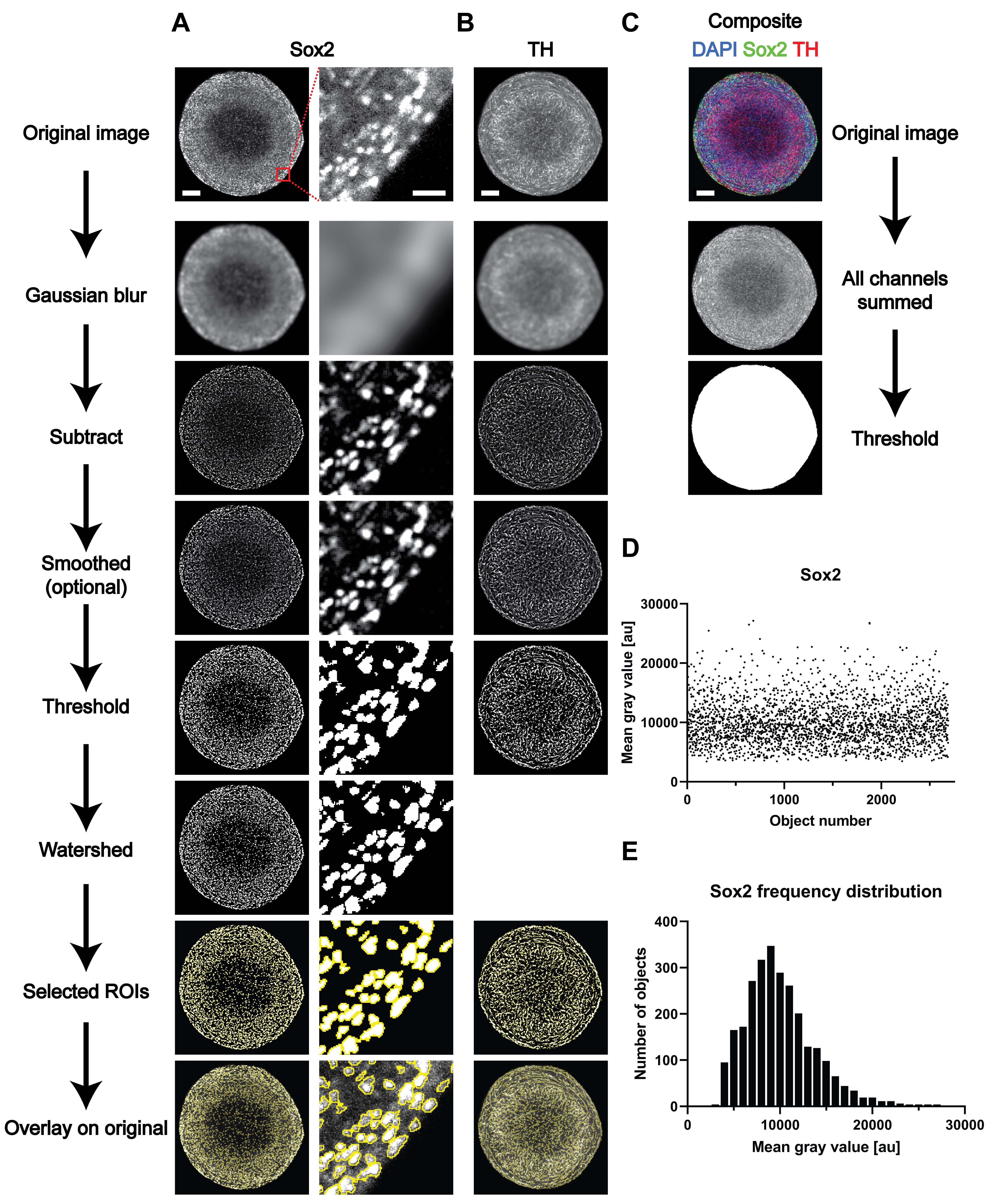
Figure 1. Overview of the different steps of image analysis of whole-mount-stained and cleared 3D structures. (A-C) Representative images of the different steps from the image analysis process outlined in the Procedure Section D. (D-E) Representative results for the analysis of the nuclear marker Sox2. (D) Raw data (i.e., mean gray value for every of the identified objects) and (E) frequency distribution based on the data shown in D). Scale bars in the top image of each row (A-C) are valid for the entire column of images below. Scale bars: entire organoids = 100 μm; enlargement (A, right column) = 20 μm.Data analysis
The manual analysis of images acquired with a confocal microscope is described under “Procedure section D: Fluorescence-based single-cell analysis.” The analysis of high-content imaging data is described in detail in the original publication (Renner et al., 2020) under “Materials and Methods,” “General workflow for high-content imaging and analysis,” and the following sections.
Notes
The BABB-based clearing procedure tends to quench the native fluorescence of fluorescent fusion proteins, including GFP, RFP, and all the mFruits. However, fluorescent dyes, including the Alexa fluors, are not affected. Thus, we recommend performing the whole-mount staining procedure outlined above using specific antibodies raised against the fluorescent protein of interest (e.g., anti-GFP) to analyze them in BABB-cleared structures. This has the additional benefit of signal amplification via multivalent secondary antibodies and better photostability, as commercial dyes commonly surpass the bleaching resistance of native fusion proteins.
Several steps of the protocol can be optimized to save antibody solution, especially in large-scale experiments. Two options that have worked well in our hands are:
Reducing the volume of the antibody solution used to a minimum of 50 μl (for large samples, it can also be increased to 200 μl or more to yield better results).
Only replacing the antibody solution once after 3 days of incubation (instead of twice, after 2 and 4 days).
Note: This is highly specific for every individual experiment and dependent, amongst other factors, on the size of the aggregates and antibodies used. Therefore, this should be carefully validated before performing larger experiments or using valuable samples.
Recipes
Permeabilization buffer (Table 1)
Table 1. Permeabilization buffer
Reagent Amount for 10 ml Supplier Product no. Dilution factor Stock conc.* PBS 9.5 ml Sigma-Aldrich D8662 Triton X-100 500 μl Roth 3051.21 20 10% (v/v) Blocking solution (Table 2)
Table 2. Blocking solution
Reagent Amount for 10 ml Supplier Product no. Dilution factor Stock conc.* PBS 1.4 ml Sigma-Aldrich D8662 BSA 8 ml Thermo Fisher 15260037 1.25 7.5% Triton X-100 500 μl Roth 3051.21 20 10% (v/v) Sodium azide 100 μl Sigma-Aldrich 71289 100 10%(w/v) *Whereas not required, we recommend preparing intermediary stock solutions of Triton X-100 (10% (v/v) in PBS) and sodium azide (10% (w/v) in PBS) as facilitates handling.
BABB/methanol (Table 3)
Table 3. BABB/methanol
Reagent Amount for 10 ml Supplier Product no. Methanol 5 ml Roth 4627.6 Benzyl alcohol 2.5 ml Sigma-Aldrich 305197-100ML Benzyl benzoate 2.5 ml Sigma-Aldrich B6630-250ML BABB (Table 4)
Table 4. BABB
Reagent Amount for 10 ml Supplier Product no. Benzyl alcohol 5 ml Sigma-Aldrich 305197-100ML Benzyl benzoate 5 ml Sigma-Aldrich B6630-250ML Note: The permeabilization buffer can be stored at room temperature for several months. The blocking solution should be stored at 4°C and can be used for approximately 1 month. BABB/methanol and BABB should be freshly prepared right before use.
Acknowledgments
This work was funded by the European Research Council (ERC) under the European Union's Horizon 2020 research and innovation program (grant agreement No [669168]). HR is supported by the International Max Planck Research School - Molecular Biomedicine, Münster, Germany. This protocol is based on our previous publication (Renner et al., 2020) (DOI: 10.7554/eLife.52904).
Competing interests
The work presented here is the subject of the patent application EP 18 19 2698.0-1120 to the European Patent Office, where all of the authors are inventors.
References
- Dekkers, J. F., Alieva, M., Wellens, L. M., Ariese, H. C. R., Jamieson, P. R., Vonk, A. M., Amatngalim, G. D., Hu, H., Oost, K. C., Snippert, H. J. G., Beekman, J. M., Wehrens, E. J., Visvader, J. E., Clevers, H. and Rios, A. C. (2019). High-resolution 3D imaging of fixed and cleared organoids. Nat Protoc 14(6): 1756-1771.
- Dent, J. A., Polson, A. G. and Klymkowsky, M. W. (1989). A whole-mount immunocytochemical analysis of the expression of the intermediate filament protein vimentin in Xenopus. Development 105(1): 61-74.
- Kim, J., Koo, B. K. and Knoblich, J. A. (2020). Human organoids: model systems for human biology and medicine. Nat Rev Mol Cell Biol 21(10): 571-584.
- Lancaster, M. A., Renner, M., Martin, C. A., Wenzel, D., Bicknell, L. S., Hurles, M. E., Homfray, T., Penninger, J. M., Jackson, A. P. and Knoblich, J. A. (2013). Cerebral organoids model human brain development and microcephaly. Nature 501(7467): 373-379.
- Lee, E., Choi, J., Jo, Y., Kim, J. Y., Jang, Y. J., Lee, H. M., Kim, S. Y., Lee, H. J., Cho, K., Jung, N., Hur, E. M., Jeong, S. J., Moon, C., Choe, Y., Rhyu, I. J., Kim, H. and Sun, W. (2016). ACT-PRESTO: Rapid and consistent tissue clearing and labeling method for 3-dimensional (3D) imaging.Sci Rep 6: 18631.
- Masselink, W., Reumann, D., Murawala, P., Pasierbek, P., Taniguchi, Y., Bonnay, F., Meixner, K., Knoblich, J. A. and Tanaka, E. M. (2019). Broad applicability of a streamlined ethyl cinnamate-based clearing procedure. Development 146(3).
- Pasca, A. M., Sloan, S. A., Clarke, L. E., Tian, Y., Makinson, C. D., Huber, N., Kim, C. H., Park, J. Y., O'Rourke, N. A., Nguyen, K. D., Smith, S. J., Huguenard, J. R., Geschwind, D. H., Barres, B. A. and Pasca, S. P. (2015). Functional cortical neurons and astrocytes from human pluripotent stem cells in 3D culture. Nat Methods 12(7): 671-678.
- Renner, H., Grabos, M., Becker, K. J., Kagermeier, T. E., Wu, J., Otto, M., Peischard, S., Zeuschner, D., TsyTsyura, Y., Disse, P., Klingauf, J., Leidel, S. A., Seebohm, G., Scholer, H. R. and Bruder, J. M. (2020). A fully automated high-throughput workflow for 3D-based chemical screening in human midbrain organoids. Elife 9: e52904.
- Rossi, G., Manfrin, A. and Lutolf, M. P. (2018). Progress and potential in organoid research. Nat Rev Genet 19(11): 671-687.
- Schindelin, J., Arganda-Carreras, I., Frise, E., Kaynig, V., Longair, M., Pietzsch, T., Preibisch, S., Rueden, C., Saalfeld, S., Schmid, B., Tinevez, J. Y., White, D. J., Hartenstein, V., Eliceiri, K., Tomancak, P. and Cardona, A. (2012). Fiji: an open-source platform for biological-image analysis. Nat Methods 9(7): 676-682.
- Schutgens, F. and Clevers, H. (2020). Human Organoids: Tools for Understanding Biology and Treating Diseases. Annu Rev Pathol 15: 211-234.
文章信息
版权信息
![]() Renner et al. This article is distributed under the terms of the Creative Commons Attribution License (CC BY 4.0).
Renner et al. This article is distributed under the terms of the Creative Commons Attribution License (CC BY 4.0).
如何引用
Readers should cite both the Bio-protocol article and the original research article where this protocol was used:
- Renner, H., Otto, M., Grabos, M., Schöler, H. R. and Bruder, J. M. (2021). Fluorescence-based Single-cell Analysis of Whole-mount-stained and Cleared Microtissues and Organoids for High Throughput Screening. Bio-protocol 11(12): e4050. DOI: 10.21769/BioProtoc.4050.
- Renner, H., Grabos, M., Becker, K. J., Kagermeier, T. E., Wu, J., Otto, M., Peischard, S., Zeuschner, D., TsyTsyura, Y., Disse, P., Klingauf, J., Leidel, S. A., Seebohm, G., Scholer, H. R. and Bruder, J. M. (2020). A fully automated high-throughput workflow for 3D-based chemical screening in human midbrain organoids. Elife 9: e52904.
分类
细胞生物学 > 细胞成像 > 固定组织成像
细胞生物学 > 细胞成像 > 共聚焦显微镜
您对这篇实验方法有问题吗?
在此处发布您的问题,我们将邀请本文作者来回答。同时,我们会将您的问题发布到Bio-protocol Exchange,以便寻求社区成员的帮助。