

Characterization of Biological Motion Using Motion Sensing Superpixels
基于运动传感超像素的生物运动特性研究
发布: 2019年09月20日第9卷第18期 DOI: 10.21769/BioProtoc.3365 浏览次数: 5941
评审: Zinan ZhouDr. Kalpa MehtaFarah Haque
参见作者原研究论文
The authors used this protocol in:

Feb 2019
Advertisement


Abstract
Precise spatiotemporal regulation is the foundation for the healthy development and maintenance of living organisms. All cells must correctly execute their function in the right place at the right time. Cellular motion is thus an important dynamic readout of signaling in key disease-relevant molecular pathways. However despite the rapid advancement of imaging technology, a comprehensive quantitative description of motion imaged under different imaging modalities at all spatiotemporal scales; molecular, cellular and tissue-level is still lacking. Generally, cells move either ‘individually’ or ‘collectively’ as a group with nearby cells. Current computational tools specifically focus on one or the other regime, limiting their general applicability. To address this, we recently developed and reported a new computational framework, Motion Sensing Superpixels (MOSES). Incorporating the individual advantages of single cell trackers for individual cell and particle image velocimetry (PIV) for collective cell motion analyses, MOSES enables ‘mesoscale’ analysis of both single-cell and collective motion over arbitrarily long times. At the same time, MOSES readily complements existing single-cell tracking workflows with additional characterization of global motion patterns and interaction analysis between cells and also operates directly on PIV extracted motion fields to yield rich motion trajectories analogous for single-cell tracks suitable for high-throughput motion phenotyping. This protocol provides a step-by-step practical guide for those interested in applying MOSES to their own datasets. The protocol highlights the salient features of a MOSES analysis and demonstrates the ease-of-use and wide applicability of MOSES to biological imaging through demo experimental analyses with ready-to-use code snippets of four datasets from different microscope modalities; phase-contrast, fluorescent, lightsheet and intra-vital microscopy. In addition we discuss critical points of consideration in the analysis.
Keywords: Biological motion (生物性运动 )Background
In general, cells exhibit two types of movement; ‘single-cell’ or ‘individual’ migration in which each cell migrates independently or ‘collective’ migration where nearby cells migrate as a group in a coordinated fashion. Current computational tools focus on one or the other regime. To date numerous single-cell tracking methods have been developed that extract the movement trajectories of individual cells to build rich motion feature descriptors suitable for the unbiased analysis of high-throughput screens (Padfield et al., 2011; Meijeringet al., 2012; Maška et al., 2014; Schiegg et al., 2015; Nketia et al., 2017). However the performance of these algorithms requires accurate delineation or segmentation and subsequent temporal association of individual identified cells between video frames. This process is unfortunately difficult to generalize across applications, requires significant expertise and computationally scales poorly with increasing cell number. Single-cell tracking thus places an inherent upper limit to the time duration that can be imaged and tracked. In contrast, collective motion analysis tools such as Particle Image Velocimetry (PIV) exploit local correlation between image patch intensity values to derive velocities for all image pixels between all pairs of frames (Szabó et al., 2006; Petitjean et al., 2010; Milde et al., 2012). Advantageously this avoids errors introduced by image segmentation, is much easier to use for non-experts and is computationally efficient, scaling only with the number of region of interests (ROI) the image is divided into. Unfortunately, despite attempts to extract more descriptive motion parameters aside from PIV velocity such as including appearance parameters (Neumann et al., 2006; Zaritsky et al., 2012; 2014; 2015 and 2017), systematic characterization of the PIV extracted velocity fields to derive similarly rich ‘signatures’ as afforded by single-cell track measurements over arbitrarily long times for clustering motion patterns within and across videos is lacking. Further investigation of how the pixel-based or ROI measurements relate to particular individual cells or cell groups in the moving collectives has also been underexplored. As such PIV based analyses have exhibited limited success when studying phenomena associated with complex cellular movement such as boundary formation and chemoattraction in-vivo.
Recently we developed Motion Sensing Superpixels (MOSES) (Zhou et al., 2019), a computational framework that marries together the ability to generate rich motion features offered by single-cell tracking trajectories with the ease-of-use and computational efficiency of segmentation-free PIV methods. MOSES achieves this by firstly extending PIV-type methods to generate long-time motion trajectories analogous to single-cell tracks for user-defined ROIs called superpixels and secondly the construction of a mesh over the extracted motion trajectories to systematically capture the spatio-temporal interaction between neighboring ROIs. This protocol through ready-to-use code snippets details how to do this practically using the previously published MOSES code as a Python library.
Equipment
- Single-channel or multi-channel time-lapse microscope, for taking videos of any modality, e.g., fluorescence, phase contrast
Note: Videos should be in one of the standard bio-formats (TIFF, STK, LSM or FluoView) or a commonly used general video format (.mp4, .avi, .mov). - Computer
Recommended PC requirements:
Processor (CPU): minimum Intel i5 2.4GHz
RAM: minimum 8GB, recommended > 16GB
Hard disk: few MBs per multi-channel image
Note: The recommended requirements are given for 1024 x 1344 RGB images. The use of smaller sized or downsampled images require less RAM and less powerful CPU specifications.
Software
- Windows/MacOS/Linux Operating system (64-bit)
- Python 2.7 or 3.6 Python Anaconda installation
- Git (https://git-scm.com/)
- Motion Sensing Superpixels (MOSES, https://github.com/fyz11/MOSES)
- Fiji ImageJ for visualization (https://fiji.sc/)
Procedure
We describe the general protocol to extract superpixel long-time trajectories and motion measurements as described in our original publication (Zhou et al., 2019). The presented code snippets in this section are also provided in the supplementary Python script file (‘general_analysis_protocol.py’) to aid re-implementation. Adaptation of the basic procedure for the analysis of different datasets acquired by different microscope modalities is detailed in the Data Analysis section. The code and protocols should work for both Python 2 and 3 installations. They were originally developed using Python 2.7 under a Linux Mint Cinnamon 17 operating system. We assume throughout basic familiarity with working with command line prompts and terminals such as folder navigation using the cd or dir commands and basic Python usage including the importing of Python modules using import, array indexing using NumPy and plotting using Matplotlib libraries.
- Protocol Nomenclature
- “Open a terminal”: refers to the launching of an appropriate terminal window on your operating system (OS) to issue command-line commands. On Windows the terminal is the command prompt or Git bash program. On Windows systems a command prompt can be launched by opening the Start Menu, typing in the search bar cmd and clicking on the command prompt logo, usually the first search result. On MacOS one can execute the shortcut key combination (⌘ + Ctrl T). On Linux systems one can execute the shortcut key combination (Ctrl-Alt T).
- Commands to be executed in a terminal are distinguished from regular text by use of the true typewriter font Courier New for example python script.py.
- <input folder>: angular brackets denote text placeholders. The user should replace the placeholder with an appropriate text string (enclosed by speech marks or without spaces) according to the prompt text written in true typewriter font within the brackets. Usually, this is the path to a particular input/output file or folder.
- Installing Python and MOSES
- Download the appropriate Python Anaconda installer for your operating system.
- Install Python Anaconda following the on-screen instruction prompts of the graphical installer to install for macOS and Windows. For Linux distributions open a terminal, execute bash <path to installer file> and proceed to follow the instructions in the terminal.
- (Optional) Create a new anaconda environment just for MOSES. Open a terminal and execute conda create --name <myenv> pip. This will create a new virtual environment with the name myenv and pip, a package manager for Python. Check the environment was successfully created by executing conda info --envs. We can now install Python software libraries only to this environment without affecting previous Python installations using conda by executing conda install <package_name> --name <myenv>. To load and use this environment execute conda activate <myenv> or source activate <myenv> in MacOS and Linux or activate myenv in Windows. For more information regarding the management of virtual environments see https://docs.conda.io/projects/conda/en/latest/user-guide/tasks/manage-pkgs.html.
Note: This optional step helps to keep all software dependencies for MOSES isolated from the rest of your Python installations. - Download the MOSES scripts from https://github.com/fyz11/MOSES. Either:
- Clone the github repository, git clone https://github.com/fyz11/MOSES.git.
- Click the green ‘Clone or download’ button. Then click ‘Download ZIP’ and extract the .zip contents.
- Install MOSES. Either:
- Install to your Python installation to make it available system wide. This can be done by executing python setup.py install in the downloaded Github folder. Installation in this manner enables the scripts to be imported and used no matter the location of your analysis scripts. If you have set up a virtual environment previously for MOSES, load the environment before executing the command.
- Copy and paste the entire contents of the ‘MOSES’ folder in the Github repository into your top-level or root project folder such that ‘MOSES’ is co-located in the same subfolder used to store the analysis scripts (Figure 1).
Note: Option a) minimizes code replication across projects whilst, option b) offers the greatest ease for prototyping and customizing the MOSES scripts.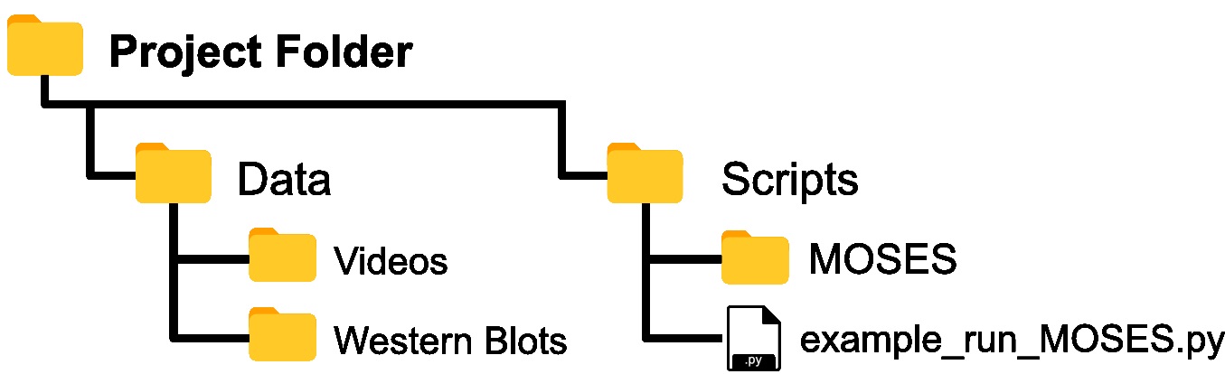
Figure 1. Assumed folder structure if copy and pasting MOSES code for installation
- Install MOSES dependencies. MOSES depends on the number of externally managed Python code libraries that needs to be installed. Using option a) (Step B5b) above automates these steps. If using option b) (Step B5b) execute pip install –r requirements.txt in the terminal loading the virtual environment before execution if required. Please note MoviePy, one of the external Python dependencies required for reading and writing general video formats depends on the FFMPEG library (https://ffmpeg.org/). This library should be automatically installed when MoviePy is installed. If this is not the case, please install manually.
Note: requirements.txt is a file in the downloaded MOSES Github repository which contains the names of all the required Python dependencies.
- Structure of the MOSES Library
The MOSES library is organized according to Figure 2. Scripts are in general organized by function. For example ‘Motion_Analysis’ contains all scripts related to the analysis of motion such as the computation of motion metrics, ‘Optical_Flow_Tracking’ contains scripts related to the computation of the motion field and the tracking of superpixels to generate superpixel tracks and ‘Utility_Functions’ contains useful scripts for file manipulation such as the reading and writing of videos. Importing of MOSES functions follow standard Python practice.
Note: Detailed documentation of each implemented function can also be browsed viewed offline by navigating to and opening the index.html file with any web browser. Within Python the normal help(<function>)can be used to read the corresponding documentation for a given function.
For the remaining sections of the protocol, we assume the exemplar folder structure in Figure 1 placing the analysis script and video data in separate folders.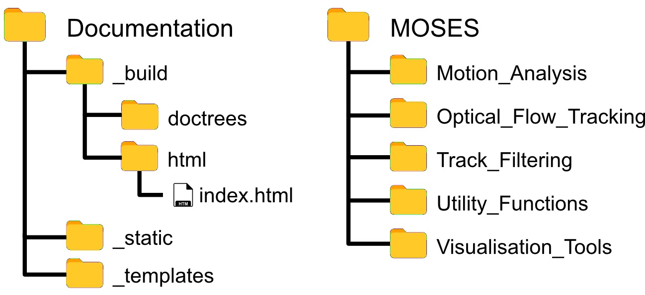
Figure 2. Folder and file structure of the MOSES Github code repository - Running Python
Several ways exist to run Python. We recommend for scientific computing the use of Spyder as an integrated development environment for scientific analysis. If not available under the current environment it can be installed using conda install –c conda-forge spyder --name <myenv>.- Launch Spyder using the terminal spyder &. The interface is similar to that of RStudio for R users (Figure 3).
- Copy and paste code snippets into the editor and save the script.
- Run the entire script using the keyboard shortcut F5 or by clicking the green ‘play’ button. Run selected lines of code using the keyboard shortcut F9.
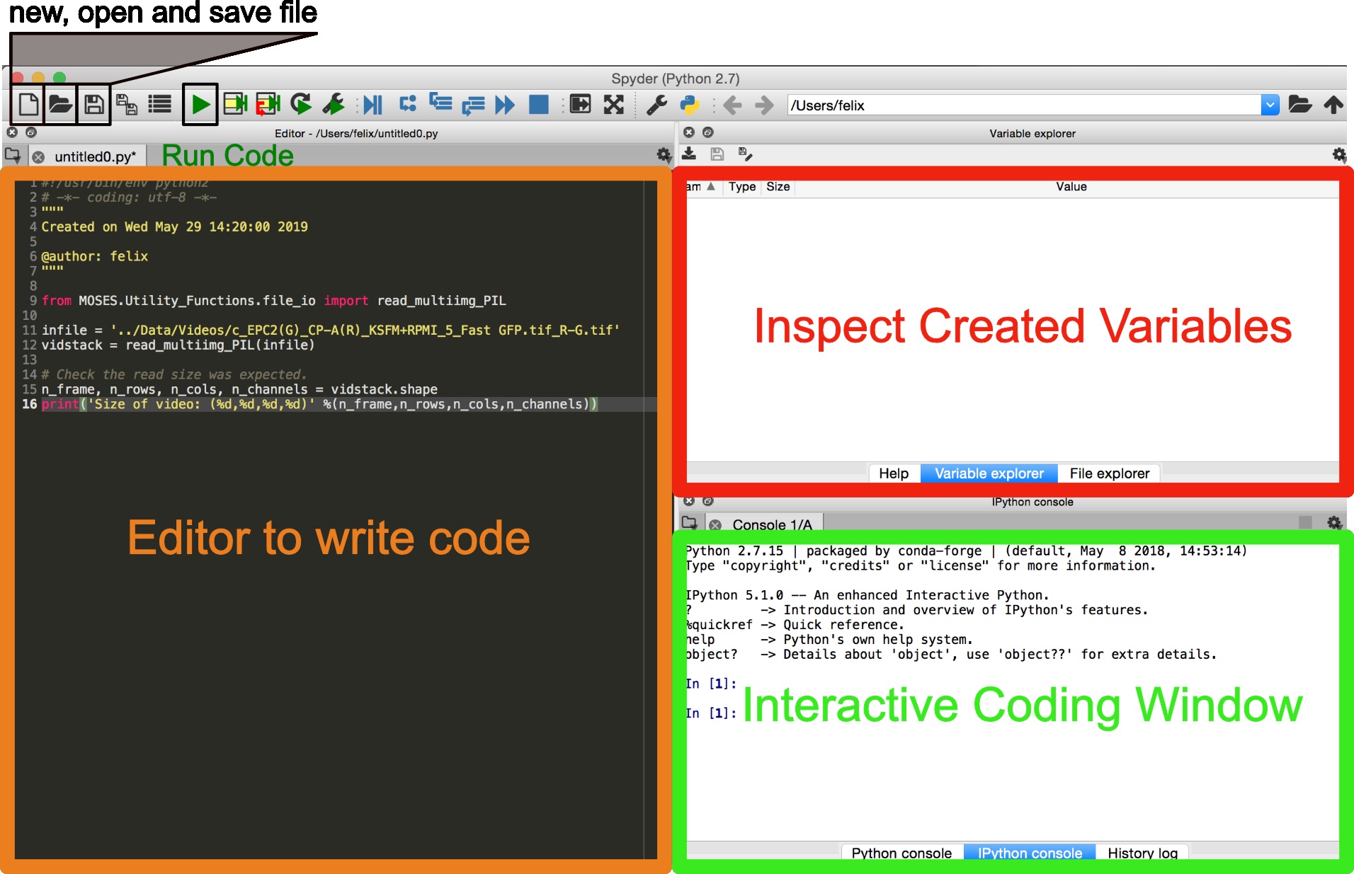
Figure 3. Graphical user interface (GUI) of Spyder for scientific programming
- Compute MOSES Superpixel Tracks
- Download the ‘c_EPC2(G)_CP-A(R)_KSFM+RPMI_5_Fast GFP.tif_R-G.tif’ video file to use as an example red-green fluorescent .tif timelapse video from the following Google Drive link and save this to a ‘Videos’ subfolder underneath the ‘Data’ folder as in Figure 1.
- Read in the video as a numpy array object by importing and using the function read_multiimg_PIL. For multi-channel videos, this gives a 4-dimensional matrix, for single-channel videos this gives a 3-dimensional matrix.
Note: More generally one can use the function read_multiimg_stack instead to read in a general bio-format image with additional z-slices.
from MOSES.Utility_Functions.file_io import read_multiimg_PIL
infile = ’../Data/Videos/c_EPC2(G)_CP-A(R)_KSFM+RPMI_5_Fast_GFP.tif_R-G.tif’
vidstack = read_multiimg_PIL(infile)
# Check the read size was expected.
n_frame, n_rows, n_cols, n_channels = vidstack.shape
print(‘Size of video: (%d,%d,%d,%d)’ %(n_frame, n_rows, n_cols, n_channels)) - Define the optical flow parameter settings used for superpixel tracking. For more details of the used Farnebäck flow computation to compute pixel velocities refer to the OpenCV documentation and the original paper (Farnebäck, 2003). The parameters determine the accuracy of the motion field computation (see Notes).
Note: Use more levels, e.g., 5, increase the winsize, e.g., 21 and increase iterations e.g., 5 to capture discontinuous movement over larger distances (with respect to input image size as measured in pixels), see also notes section of this protocol.
optical_flow_params = dict(pyr_scale=0.5, levels=3, winsize=15, iteratons=3, poly_n=5, poly_sigma=1.2, flags=0) - Specify the target number of superpixels or square region of interests (ROI) to subdivide the video frame. For an image size of n × m pixels, a specification of N superpixels would yield individual superpixels with an approximate size of
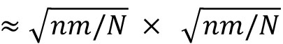 pixels. For n=512,m=512,N=1000, each superpixel will be of size ≈16×16 pixels.
# number of superpixels
n_spixels = 1000 - For each image channel, extract the superpixel tracks and the computed motion field noting the 0-indexing.
from MOSES.Optical_Flow_Tracking.superpixel_track import compute_grayscale_vid_superpixel_tracks
# extract superpixel tracks for the 1st or ‘red’ channel
optflow_r, meantracks_r = compute_grayscale_vid_superpixel_tracks(vidstack[:,:,:,0], optical_flow_params, n_spixels)
# extract superpixel tracks for the 2nd or ‘green’ channel
optflow_g, meantracks_g = compute_grayscale_vid_superpixel_tracks(vidstack[:,:,:,1], optical_flow_params, n_spixels) - Save the computed tracks in .mat MATLAB format. Alternative formats that support Python array saving can be used such as Python pickle or HDF.
import scipy.io as spio
import os
fname = os.path.split(infile)[-1]
savetracksmat = (‘meantracks_’ + fname).replace(‘.tif’, ‘.mat’)
spio.savemat(savetracksmat, {‘meantracks_r’:meantracks_r, ‘meantracks_g’: meantracks_g})
- (Optional) Visualize the motion field for select frames to check the computation (Figure 4) and optionally save the computed motion field.
Note: For large images saving the motion field takes up a lot of hard disk space. It is therefore not recommended to do so. The motion field is summarized by the superpixel tracks.
import pylab as plt
from MOSES.Visualisation_Tools.motion_field_visualisation import view_ang_flow
# visualize first frame of red and green motion fields
fig, ax = plt.subplots(nrows=1, ncols=2)
ax[0].imshow(view_ang_flow(optflow_g[0]))
ax[1].imshow(view_ang_flow(optflow_r[0]))
ax[0].grid(‘off’); ax[1].grid(‘off’)
plt.show()
# save the flow
save_optflow_mat = (‘optflow_’+fname).replace(‘.tif’, ‘.mat’)
spio.savemat(save_optflow_mat, {‘optflow_r’: optflow_r, ‘optflow_g’: optflow_g})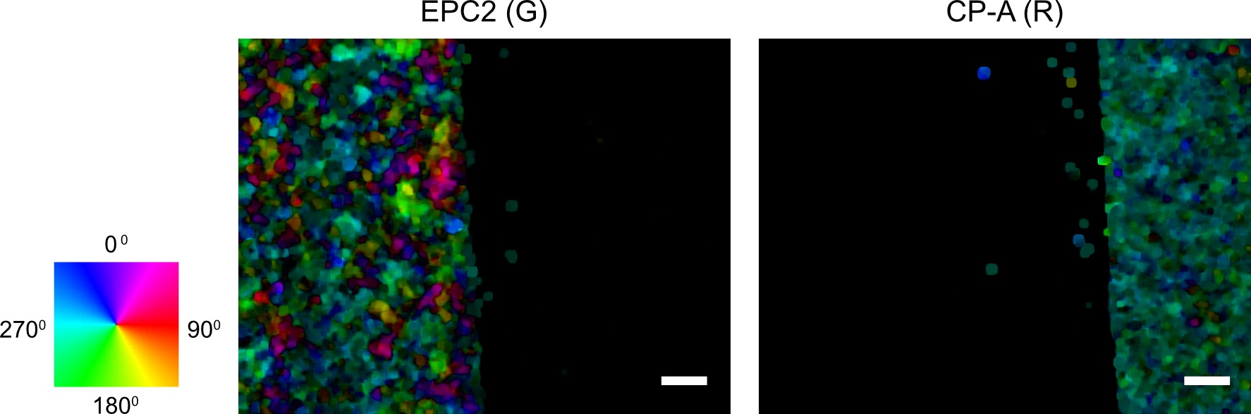
Figure 4. Visualization of the computed first frame motion field using optical flow for red and green channel images. The individual pixel velocities are colored by their angular direction using the color wheel with the color intensity encoding the pixel speed. Scale bars: 200 µm. - (Optional) Plot the superpixel tracks as a second sanity check. The shape of the tracks should capture the dynamic range of the moving entities in the video. For epithelial sheets, this is the shape of the leading edge of the sheet (Figure 5).
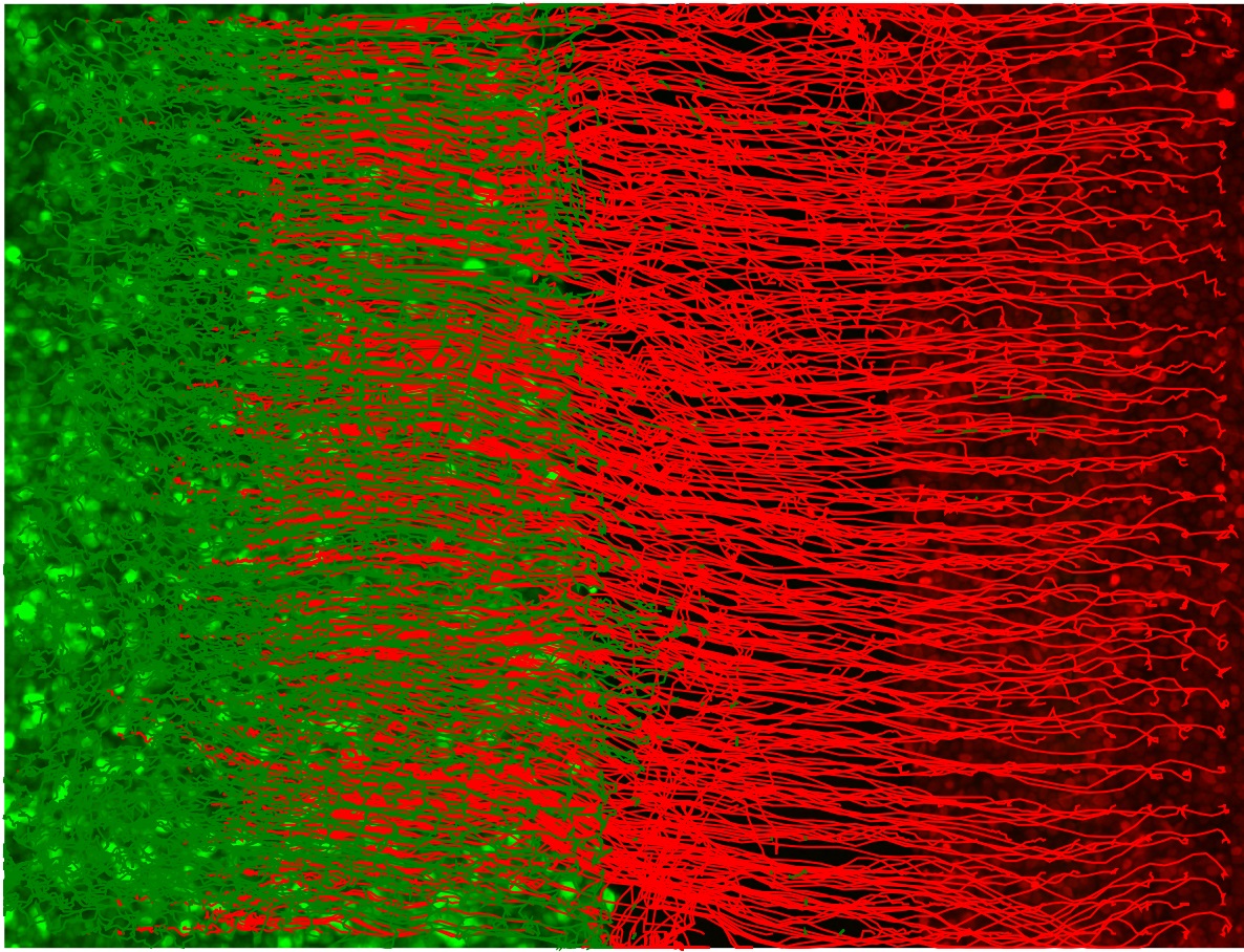
Figure 5. Plot of the red and green channel superpixel tracks. The green EPC2 tracks end on the right where it met the red CP-A tracks and was pushed back to the left. The red CP-A tracks end on the left at the final position where it has pushed the green EPC2 cells to. - (Optional for debugging) Produce a video of the superpixel tracks overlaid on the video, plotting each track in temporal segments of 5 frames to avoid clutter. Frames are generated sequentially. Subsequently, import the saved frames using Fiji ImageJ in temporal order, File → Import → Image Sequence... and save as a multipage .tif video (File → Save As → Tiff...) or .avi video, (File → Save As → AVI...).
from MOSES.Utility_Functions.file_io import mkdir
from MOSES.Visualisation_Tools.track_plotting import plot_tracks
import os
fname = os.path.split(infile)[-1]
# specify the save folder and create this automatically.
save_frame_folder = ‘track_video’
mkdir(save_frame_folder)
len_segment = 5
for frame in range(len_segment, n_frame, 1):
frame_img = vidstack[frame]
fig = plt.figure()
fig.set_size_inches(float(n_cols)/n_rows, 1, forward=False)
ax=plt.Axes(fig, [0.,0.,1.,1.]); ax.set_axis_off(); fig.add_axes(ax)
ax.imshow(frame_img, alpha=0.6)
# visualize only a short segment
plot_tracks(meantracks_r[:,frame-len_segment:frame+1],ax, color='r', lw=1)
plot_tracks(meantracks_g[:,frame-len_segment:frame+1],ax, color='g', lw=1)
ax.set_xlim([0, n_cols]); ax.set_ylim([n_rows, 0])
ax.grid('off'); ax.axis('off')
# tip: use multiples of n_rows to increase image resolution
fig.savefig(os.path.join(save_frame_folder, 'tracksimg-%s_' %(str(frame+1).zfill(3))+fname.replace('.tif','.png')), dpi=n_rows)
plt.show()
- Construct Mesh from Superpixel Tracks
Any individual moving entity inevitably affects the motion of surrounding entities. Considering superpixels as individual moving elements, it becomes natural to capture the interaction between each superpixel and its neighbors. Computationally this interaction can be captured in a mesh or graph with mesh edges representing the presence of an interaction. This mesh construction critically depends on what one considers evidence of interaction or motion similarity. As such different meshes can be constructed to better highlight different aspects of the cellular motion. We direct the interested reader to the supplementary information of Zhou et al., 2019 for an extended discussion. Below we describe the construction steps for three meshes which connect together superpixel tracks based on different notions of spatial proximity.- Construct the MOSES mesh for individual image channels by connecting each superpixel track to all superpixel tracks separated by at most a pixel distance less than a multiple (dist_thresh) of the average superpixel width (spixel_size) based on the initial (x,y) position of superpixels.
Note: The MOSES mesh captures how superpixels move with respect to their initial neighbors.
from MOSES.Motion_Analysis.mesh_statistics_tools import construct_MOSES_mesh
# specify the average superpixel size. This is roughly the width for squares
spixel_size = meantracks_r[1,0,1] - meantracks_r[1,0,0]
# compute the MOSES mesh, linking together all superpixels located a distance dist_thresh*spixel_size for each colour channel
MOSES_mesh_strain_time_r, MOSES_mesh_neighborlist_r = construct_MOSES_mesh(meantracks_r, dist_thresh=1.2, spixel_size=spixel_size)
MOSES_mesh_strain_time_g, MOSES_mesh_neighborlist_g = construct_MOSES_mesh(meantracks_g, dist_thresh=1.2, spixel_size=spixel_size) - Construct the radial neighbors mesh for individual image channels by connecting each superpixel track to all superpixel tracks at time t separated by at most a pixel distance less than a multiple (dist_thresh) of the average superpixel width (spixel_size) based on the (x,y) position of the superpixels at time t.
Note: Unlike the MOSES mesh, the connections between neighbors in the radial neighbor mesh dynamically changes over time.
from MOSES.Motion_Analysis.mesh_statistics_tools import construct_radial_neighbour_mesh
radial_mesh_strain_time_r, radial_neighbourlist_time_r = construct_radial_neighbour_mesh(meantracks_r, dist_thresh=1.2, spixel_size=spixel_size, use_counts=False)
radial_mesh_strain_time_g, radial_neighbourlist_time_g = construct_radial_neighbour_mesh(meantracks_g, dist_thresh=1.2, spixel_size=spixel_size, use_counts=False) - Construct the K nearest neighbor mesh for individual image channels by connecting each superpixel track to the K superpixel tracks at time t that is spatially closest based on the (x,y) position of the superpixels at time t.
Note: This mesh is constructed based on topological distance and is suitable when the physical spatial separation is not a significant factor.
from MOSES.Motion_Analysis.mesh_statistics_tools import construct_knn_neighbour_mesh
knn_mesh_strain_time_r, knn_neighbourlist_time_r = construct_knn_neighbour_mesh(meantracks_r, k=4)
knn_mesh_strain_time_g, knn_neighbourlist_time_g = construct_knn_neighbour_mesh(meantracks_g, k=4) - (Optional) Visualize the constructed mesh at select frames (here for example frame 20) to check construction (Figure 6). The example code visualizes the MOSES mesh from Step F1. Any mesh specified either as a networkx graph object or as a list specifying the array index of superpixels connected to each superpixel i can similarly be visualized.
from MOSES.Visualisation_Tools.mesh_visualisation import visualize_mesh
from MOSES.Motion_Analysis.mesh_statistics_tools import from_neighbor_list_to_graph
# use networkx to visualize the mesh at frame 20. To do so need to first convert the neighborlist into a networkx graph object.
mesh_frame20_networkx_G_red = from_neighbor_list_to_graph(meantracks_r, MOSES_mesh_neighborlist_r, 20)
mesh_frame20_networkx_G_green = from_neighbor_list_to_graph(meantracks_g, MOSES_mesh_neighborlist_g, 20)
# set up a 1 x 2 plotting canvas.
fig, ax = plt.subplots(nrows=1, ncols=2, figsize=(15,15))
# plot the red mesh in left panel.
ax[0].imshow(vidstack[20], alpha=0.7)
visualise_mesh(mesh_frame20_networkx_G_red, meantracks_r[:,20,[1,0]], ax[0], node_size=20, linewidths=1, width=1, node_color=’r’)
ax[0].set_ylim([n_rows,0])
ax[0].set_xlim([0,n_cols])
ax[0].grid(’off’); ax[0].axis(’off’)
# plot the green mesh in right panel.
ax[1].imshow(vidstack[20], alpha=0.7)
visualise_mesh(mesh_frame20_networkx_G_green, meantracks_g[:,20,[1,0]], ax[1], node_size=20, linewidths=1, width=1, node_color=’g’)
ax[1].set_ylim([n_rows,0])
ax[1].set_xlim([0,n_cols])
ax[1].grid(’off’); ax[1].axis(’off’)
- Construct the MOSES mesh for individual image channels by connecting each superpixel track to all superpixel tracks separated by at most a pixel distance less than a multiple (dist_thresh) of the average superpixel width (spixel_size) based on the initial (x,y) position of superpixels.
- Extracting MOSES motion measurements
Several motion metrics were proposed in the original paper (Zhou et al., 2019). Here we show how to compute the main proposed metrics using the provided functions in MOSES.- Construct the motion saliency map for each color. The motion saliency map reveals spatial regions of significant motion concentration. It is computed by accumulating the mesh deformation strain in local spatial regions across time.
from MOSES.Motion_Analysis.mesh_statistics_tools import compute_motion_saliency_map
final_saliency_map_r, spatial_time_saliency_map_r = compute_motion_saliency_map(meantracks_r, dist_thresh=5.*spixel_size, shape=(n_rows, n_cols), filt=1, filt_size=spixel_size)
final_saliency_map_g, spatial_time_saliency_map_g = compute_motion_saliency_map(meantracks_g, dist_thresh=5.*spixel_size, shape=(n_rows, n_cols), filt=1, filt_size=spixel_size)
- Compute the boundary formation index from the motion saliency map. The boundary formation index is defined as the normalized ratio of the mean motion saliency map intensity values, I in high intensity image regions over low intensity image regions (‘red’ and ‘blue’ areas in Figure 7A). The intensity cut-off is automatically determined via Otsu thresholding so that a pixel with image coordinate (i,j) is in the ‘high’ region if I(i,j)≥I_thresh or else is ‘low’. The boundary formation index takes values between 0 and 1. The higher the value, the greater the propensity of motion to be concentrated within a particular spatial region.
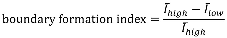
Note: Cells moving out of the field of view of the video cause superpixels to concentrate at the boundary of the videos. This causes an artefactual increase in motion density at image edges. To minimize this effect, the boundary formation index is computed in the region at least a pad_multiple times spixel_size away from the image boundary.
from MOSES.Motion_Analysis.mesh_statistics_tools import compute_boundary_formation_index
boundary_formation_index, av_saliency_map = compute_boundary_formation_index(final_saliency_map_r, final_saliency_map_g, spixel_size, pad_multiple=3)
fig = plt.figure()
plt.title('Boundary Formation Index %.3f' %(boundary_formation_index))
plt.imshow(av_saliency_map, cmap='coolwarm')
plt.axis('off'); plt.grid('off')
plt.show()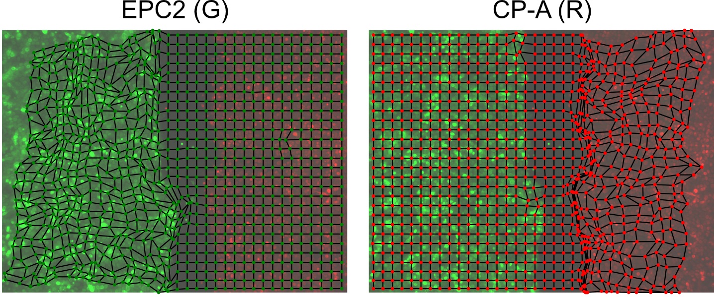
Figure 6. Visualization of the constructed MOSES mesh linking individual superpixels with centroids represented by dots - Compute the MOSES mesh strain curve of the video, the mean of curves of the individual red and green channel curves (Figure 7B). The mesh strain curve measures the mean change in the relative spatial arrangement (topology) between neighboring superpixels over time.
from MOSES.Motion_Analysis.mesh_statistics_tools import compute_MOSES_mesh_strain_curve
import numpy as np
# set normalise=True to obtain normalised curves between 0-1.
mesh_strain_r=compute_MOSES_mesh_strain_curve(MOSES_mesh_strain_time_r, normalise=False)
mesh_strain_g=compute_MOSES_mesh_strain_curve(MOSES_mesh_strain_time_g, normalise=False)
# average the channel curves to get one curve for the video.
mesh_strain_curve_video = .5*(mesh_strain_r+mesh_strain_g)
# normalise the curves, this is equivalent to normalise=True above for a single channel.
normalised_mesh_strain_curve_video = mesh_strain_curve_video/ np.max(mesh_strain_curve_video) - Compute the mesh stability index defined as 1 minus the normalized gradient of the mesh strain curve, y over a small time window, ΔT at the end of the video motion (in the interval [T,T+ΔT]). Here the time window is ΔT=5 frames (Figure 7B).
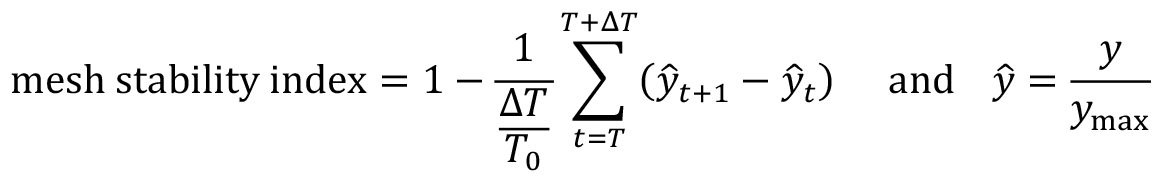
where ymax is the maximum value of the mesh strain curve and T0 is the total number of video frames. The mesh stability index is upper bounded by 1. For the example video, you should get a value of 0.892.
from MOSES.Motion_Analysis.mesh_statistics_tools import compute_MOSES_mesh_stability_index
# the mesh stability index uses an average over the last number of frame specified by the flag, last_frames. One should set this to approximately cover the plateau region of the strain curve.
mesh_stability_index, normalised_mesh_strain_curve = compute_MOSES_mesh_stability_index(MOSES_mesh_strain_time_r, MOSES_mesh_strain_time_g, last_frames=5)
print('mesh stability index: %.3f' %(mesh_stability_index))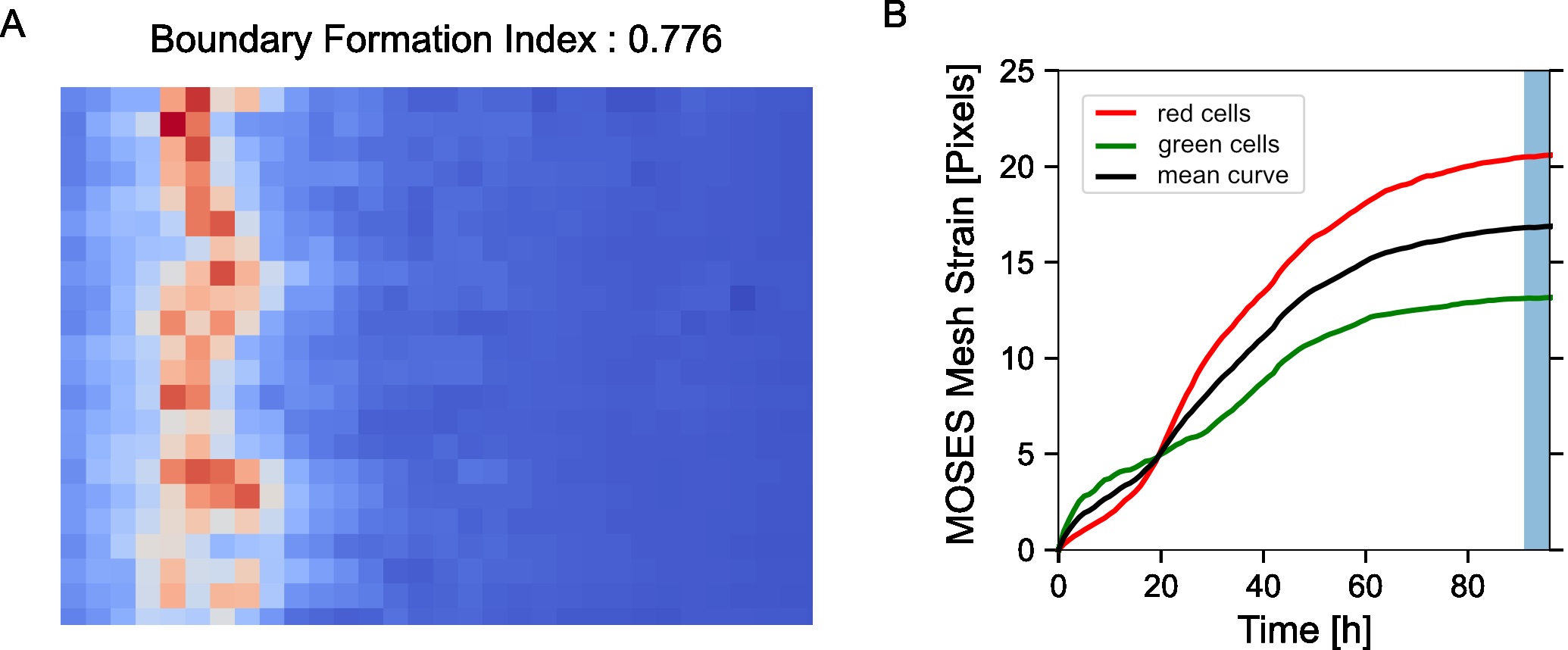
Figure 7. Motion saliency map, boundary formation index and mesh stability metrics. A. Computed motion saliency map and associated boundary formation index. B. Non-normalized MOSES mesh strain curve for red and green cell populations together with the average of the two curves (black line). Shaded blue region shows the 5 frame window used to compute the mesh stability index. - Compute the mesh strain vector. The mesh strain vector of each superpixel i is the vector sum of the displacements of neighboring superpixels j relative to the superpixel i in the mesh.
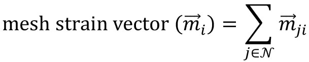
from MOSES.Motion_Analysis.mesh_statistics_tools import construct_mesh_strain_vector
# given a mesh as a list of neighbours (also known as a region adjacency list), find the mesh strain vector
mesh_strain_vector_r = construct_mesh_strain_vector(meantracks_r, [MOSES_mesh_neighborlist_r])
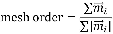
mesh_strain_vector_g = construct_mesh_strain_vector(meantracks_g, [MOSES_mesh_neighborlist_r]) - Compute the mesh order. The mesh order is the mean normalized mesh strain vector over all superpixels i, (Figure 8A). If all mesh strain vectors were aligned in the same direction, this value is 1. If there is no alignment it is 0. For the example video you should get 0.00325 (Figure 8B).
from MOSES.Motion_Analysis.mesh_statistics_tools import compute_mesh_order
mesh_order_curve_r = compute_mesh_order(mesh_strain_vector_r, remove_mean=False)
mesh_order_curve_g = compute_mesh_order(mesh_strain_vector_g, remove_mean=False)
av_mesh_order = .5*(mesh_order_curve_r + mesh_order_curve_g)
print('average mesh order: %.5f' %(np.nanmean(av_mesh_order)))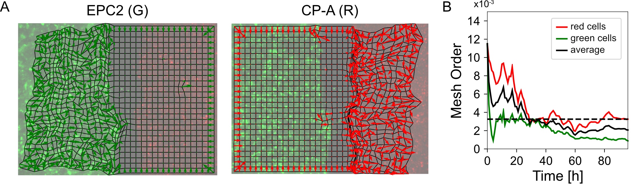
Figure 8. Visualization of the mesh order and mesh order curve. A. Mesh strain vector (colored arrows) of individual superpixels (mesh vertices) for each colored cell population overlaid on top of the MOSES mesh for frame 20. B. Evolution of the mesh order over time for individual colored populations and the average of the two colored curves (black line). Dashed black line is the mean value of all temporal values reported as the mean mesh order for the video.
- Construct the motion saliency map for each color. The motion saliency map reveals spatial regions of significant motion concentration. It is computed by accumulating the mesh deformation strain in local spatial regions across time.
Data analysis
The demo analyses presented in this section expands upon the general protocol detailed above by walking through the standard steps of motion analysis using MOSES on various different biological imaging datasets. The steps below illustrate how to adapt and work with MOSES to handle a breadth of different datasets. The analyses are additionally provided as supplementary Python script files (.py).
Analysis 1: Single Cell Tracking (Phase Contrast Microscopy) (Supplementary files)
We use the data from the Cell Tracking Challenge (http://celltrackingchallenge.net/) to illustrate how to use MOSES for single cell tracking analysis. As cell division is not currently explicitly modeled within the motion extraction in MOSES, this analysis is most effective for videos where cell proliferation is minimal or when extraction of the global ‘motion’ pattern is more important.
- Register for a free account at http://celltrackingchallenge.net/registration/, the official challenge website to download the datasets.
- Download the U373 cell training dataset from http://celltrackingchallenge.net/2d-datasets/.
- Unzip the downloaded ‘PhC-C2DH-U373.zip folder’. You should find 4 folders, ‘01’, ‘01_GT’, ‘02’ and ‘02_GT’ which specify two image sequences and their associated annotated ground truth (GT). We will only use the image sequence in ‘01’ as an example.
- Load and concatenate the image frames of ‘01’ in Python into a numpy array. The result should be a (115, 520, 696) size NumPy array.
from skimage.exposure import rescale_intensity
import numpy as np
from MOSES.Utility_Functions.file_io import detect_files
from skimage.io import imread
vid_folder = '../Data/Videos/PhC-C2DH-U373/01'
# load individal video frames saved as .tif files.
video_files, video_fnames = detect_files(vid_folder, ext='.tif')
# read individual frames and concatenate frames after rescaling intensity
vidstack = np.concatenate([rescale_intensity(imread(f))[None,:] for f in video_files], axis=0)
- Compute the superpixel tracks using n_spixels = 1000, (Figure 9A). Here we use compute_grayscale_vid_superpixel_tracks_FB to extract additional ‘backward’ tracks as a result of applying tracking running the video backward in time. Forward tracking reveals where motion flows towards (sinks) whilst backward tracking reveals spatial origins (sources) of motion, see advanced analysis section below.
Note: How will the superpixel tracks change when we increase or decrease n_spixels?
from MOSES.Optical_Flow_Tracking.superpixel_track import compute_grayscale_vid_superpixel_tracks_FB
import scipy.io as spio
n_spixels = 1000
# set the motion extraction parameters
opt_flow_params = {'pyr_scale':0.5, 'levels':7, 'winsize':25, 'iterations':3, 'poly_n':5, 'poly_sigma':1.2, 'flags':0}
# compute superpixel tracks
optflow, tracks_F, tracks_B = compute_grayscale_vid_superpixel_tracks_FB(vidstack, opt_flow_params, n_spixels=n_spixels)
# save the tracks
spio.savemat('vid01_%d_spixels.mat' %(n_spixels), {'tracks_F': tracks_F, 'tracks_B': tracks_B}) - To track cells present in the initial frame over time segment the individual cells automatically using image thresholding and connected component analysis or by manual annotation. In the paper (Zhou et al., 2019) manual annotation was used, here we use automated image thresholding (Figure 9B).
Note: Exact segmentation is not required although the more accurate the segmentation, generally the better the specificity of tracking. Results are nevertheless stable for less optimal segmentations. How are the results if bounding boxes were used?
from skimage.filters import threshold_otsu, threshold_triangle
from skimage.measure import label
from skimage.morphology import remove_small_objects, binary_closing, disk
from scipy.ndimage.morphology import binary_fill_holes
import pylab as plt
# first frame of video
frame0 = vidstack[0]
# basic quick cell segmentation by thresholding intensities
# a) determine intensity threshold
thresh = np.mean(frame0) + .5*np.std(frame0)
binary = frame0 >= thresh
# b) steps to refine the basic thresholding of a)
binary = remove_small_objects(binary, 200)
binary = binary_closing(binary, disk(5))
binary = binary_fill_holes(binary)
binary = remove_small_objects(binary, 1000)
# c) connected component analysis to label binary cell segmentation with integers
cells_frame0 = label(binary) - Use the segmentation mask to assign superpixel tracks to each segmented cell (Figure 9).
# define a function 'assign_spixels' that can be called to assign superpixel tracks using an integer labelled mask
def assign_spixels(spixeltracks, mask):
uniq_regions = np.unique(mask)
initial_pos = spixeltracks[:,0,:]
bool_mask = []
# starts from 1-index not 0-index as the first is assigned to the background.
for uniq_region in uniq_regions[1:]:
mask_region = mask == uniq_region
bool_mask.append(mask_region[initial_pos[:,0], initial_pos[:,1]])
bool_mask = np.vstack(bool_mask)
return bool_mask
cell_spixels = assign_spixels(tracks_F, cells_frame0) - Select the longest track as summary of the cell’s motion for each segmented cell region (Figure 9C).
Note: Experiment with other ways to summarize the collection of tracks into one track such as taking the mean or median of the tracks.
def find_characteristic_motion(tracks):
# This function chooses the single longest superpixel track to summarise the single cell motion.
disps_tracks = tracks[:, 1:, :] - tracks[:, :-1, :]
disps_mag = np.sum(np.sqrt(disps_tracks[:,:,0]**2 + disps_tracks[:,:,1]**2), axis=1)
rank = np.argsort(disps_mag)[::-1]
return tracks[rank[0]]
single_cell_tracks = []
# iterate through each segmentation and store the single track
for i in range(len(cell_spixels)):
# for cell i which superpixel ids belong capture it
cell_spixel = cell_spixels[i]
# for cell i retrieve the corresponding tracks
cell_tracks = tracks_F[cell_spixel]
# find the single track that summarise the motion of all associated superpixel tracks
single_cell_track = find_characteristic_motion(cell_tracks)
single_cell_tracks.append(single_cell_track[None,:])
single_cell_tracks = np.vstack(single_cell_tracks) - Visualize the inferred cell tracks, plotting each cell track with a unique color (Figure 9C).
from MOSES.Visualisation_Tools.track_plotting import plot_tracks
import seaborn as sns
cell_colors = sns.color_palette('Set1',n_colors=len(single_cell_tracks))
fig, ax = plt.subplots()
plt.title('Single Cell Tracks', fontsize=16)
ax.imshow(vidstack[0], cmap='gray')
for ii in range(len(single_cell_tracks)):
single_cell_track = single_cell_tracks[ii]
plot_tracks(single_cell_track[None,:], ax, color=cell_colors[ii], lw=3)
plt.grid('off'); plt.axis('off')
plt.show()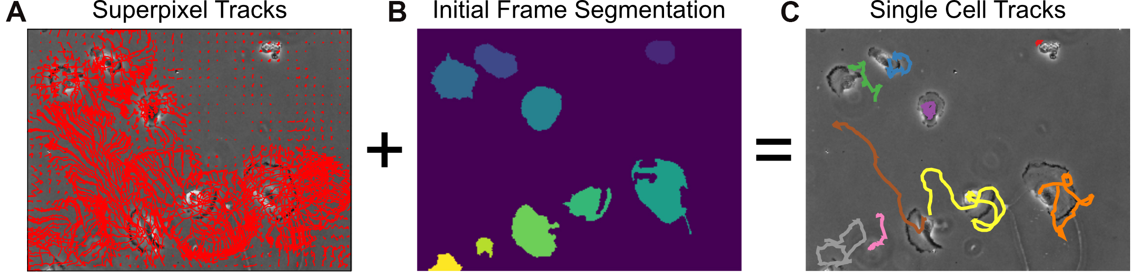
Figure 9. Single-cell tracking using MOSES superpixel tracks. A. Extracted superpixel tracks using a target number of 1,000 superpixels overlaid on the first video frame. B. Automatically segmented cells from the initial frame. C. Predicted single cell tracks selecting the longest superpixel track for each segmented cell region.Advanced analysis:
- Compute the motion saliency map using the forward and backward tracks to visualize where the cells move to and from where (Figure 10).
Note: Try changing the dist_thresh used to see how this affects the computed motion saliency map.
from MOSES.Motion_Analysis.mesh_statistics_tools import compute_motion_saliency_map
from skimage.filters import Gaussian
dist_thresh = 30
spixel_size = tracks_B[1,0,1]-tracks_B[1,0,0]
saliency_F, saliency_spatial_time_F = compute_motion_saliency_map(tracks_F, dist_thresh=dist_thresh, shape=frame0.shape, max_frame=None, filt=1, filt_size=spixel_size)
saliency_B, saliency_spatial_time_B = compute_motion_saliency_map(tracks_B, dist_thresh=dist_thresh, shape=frame0.shape, max_frame=None, filt=1, filt_size=spixel_size)
# Use Gaussian smoothing to create a more continuous heatmap
saliency_F_smooth = gaussian(saliency_F, spixel_size/2)
saliency_B_smooth = gaussian(saliency_B, spixel_size/2)
fig, ax = plt.subplots(nrows=1, ncols=3, figsize=(15,15))
ax[0].set_title('Superpixel Tracks')
ax[0].imshow(frame0, cmap='gray')
plot_tracks(tracks_F, ax=ax[0], color='r'); ax[0].axis('off')
ax[1].set_title('Motion Saliency (Forward)')
ax[1].imshow(vidstack[-1], cmap='gray')
ax[1].imshow(saliency_F_smooth, cmap='coolwarm', alpha=0.7); ax[1].axis('off')
ax[2].set_title('Motion Saliency (Backward)')
ax[2].imshow(frame0, cmap='gray')
ax[2].imshow(saliency_B_smooth, cmap='coolwarm', alpha=0.7); ax[2].axis('off')
plt.show()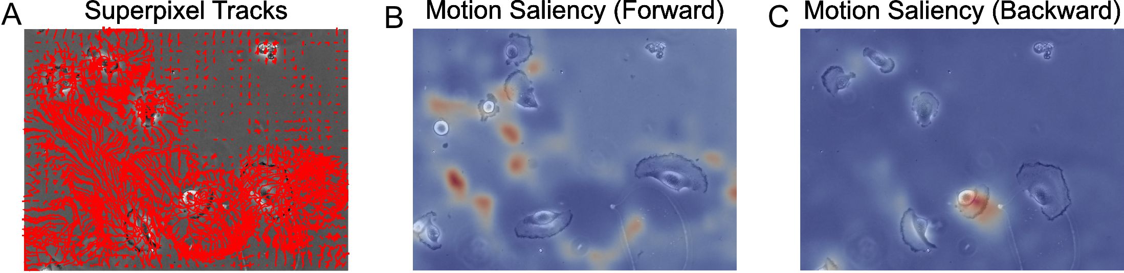
Figure 10. Motion saliency maps computed using forward and backward tracks visually uncover motion sinks and sources respectively in cellular videos. A. Extracted forward superpixel tracks using a target number of 1,000 superpixels overlaid on the first video frame. B. Forward motion saliency map computed using the forward tracks on the left reveals motion highlights the highly dynamic movement of individual cell boundaries which behave akin to motion ‘sinks’. C. Backward motion saliency map computed using the backward tracks produced tracking the video in reverse reveals motion origin or ‘sources’.
Analysis 2: Two Cell Epithelial Sheet Analysis (Fluorescence Microscopy) (Supplementary files) The main analysis steps for the migration pattern of two color epithelial sheets acquired as presented in our previous work (Zhou et al., 2019) were documented in the main protocol section. Here we present extended procedures more specifically targeted for the analysis of two-color epithelial sheets.
- Analysis of the interface between two cell populations
- Visualize the interface appearance using video kymographs. A kymograph is a projection of the 2D temporal dataset that collapses one of the spatial dimensions to allow the movement to be visualized as an image. Here the maximum along of each image pixel column was taken to summarise the motion along the image rows (Figure 11). The maximum was used to get the strongest possible signal for the interface.
from MOSES.Visualisation_Tools.kymographs import kymograph_img
import numpy as np
import pylab as plt
# project and collapse in the 'y' direction (rows)
vid_max_slice = kymograph_img(vidstack, axis=1, proj_fn=np.max)
fig, ax = plt.subplots()
ax.imshow(vid_max_slice)
ax.set_aspect('auto')
plt.show() - Visualize the interface movement between the two cell populations using velocity kymographs. Analogous to video kymographs above, velocity kymographs compress the 2D temporal motion field in one dimension to visualize the information as a single image. Here we take the median x-direction velocity value along each image pixel column to summarize the velocity variation across the rows. The median was used for projecting the information as it is an average statistic that is well-known to be robust to outlier values. MOSES provides two functions to compute the velocity kymograph depending on whether the input is a motion field or motion tracks.
- Compute the velocity kymograph of the pixel motion field (Figure 12A).
import scipy.io as spio
# load the previously computed motion field
save_optflow_mat = ('optflow_'+fname).replace('.tif', '.mat')
optflow_r = spio.loadmat(save_optflow_mat)['optflow_r']
optflow_g = spio.loadmat(save_optflow_mat)['optflow_g']
# construct the full motion field
optflow = optflow_r + optflow_g
# take only the 'x' component
optflow_x = optflow[...,0]
# kymograph 1: Dense optical flow.
optflow_median_slice = kymograph_img(optflow_x, axis=1, proj_fn=np.nanmedian) - Compute the velocity kymograph of the superpixel tracks following tracking of a fixed number of superpixels, here 1,000 superpixels, (Figure 12B).
from MOSES.Visualisation_Tools.kymographs import construct_spatial_time_MOSES_velocity_x
# load the previously computed superpixel tracks
savetracksmat = ('meantracks_'+fname).replace('.tif', '.mat')
meantracks_r = spio.loadmat(savetracksmat)['meantracks_r']
meantracks_g = spio.loadmat(savetracksmat)['meantracks_g']
# kymograph 2: Superpixel tracks. (fixed superpixel number)
velocity_kymograph_x_tracks_r = construct_spatial_time_MOSES_velocity_x(meantracks_r, shape=(n_frame, n_cols), n_samples=51, axis=1)
velocity_kymograph_x_tracks_g = construct_spatial_time_MOSES_velocity_x(meantracks_g, shape=(n_frame, n_cols), n_samples=51, axis=1)
velocity_kymograph_x_tracks = velocity_kymograph_x_tracks_r + velocity_kymograph_x_tracks_g - (Optional) Compute the velocity kymograph using the superpixel tracks extracted by dense superpixel tracking, (Figure 12C). Starting from an initial user-specified number of N superpixels, dense tracking continuously monitors the spatial density of superpixels frame to frame. The image area is regularly partitioned into N region of interests (ROI). If an ROI contains a number of superpixels less than the minimum number specified by the mindensity parameter, a new superpixel is dynamically added to the ROI and tracked in all subsequent frames. As such starting from N=1000 superpixels, the final number of superpixel tracks is variable. It could be 2,000 for videos with relatively little movement or even 6,000 for significant movement.
Note: Dense superpixel tracking is the preferred tracking approach when one expects the video to contain significant movement and is set by specifying dense=True.
# compute dense tracks by setting dense=True (default is False)
_, meantracks_r_dense = compute_grayscale_vid_superpixel_tracks(vidstack[:,:,:,0], optical_flow_params, n_spixels, dense=True, mindensity=1)
_, meantracks_g_dense = compute_grayscale_vid_superpixel_tracks(vidstack[:,:,:,1], optical_flow_params, n_spixels, dense=True, mindensity=1)
# save the computed tracks
savetracksmat = ('meantracks-dense_'+fname).replace('.tif', '.mat')
spio.savemat(savetracksmat, {'meantracks_r':meantracks_r_dense,
'meantracks_g':meantracks_g_dense})
# kymograph 3: using dense superpixel tracking.
velocity_kymograph_x_tracks_r_dense = construct_spatial_time_MOSES_velocity_x(meantracks_r_dense, shape=(n_rows, n_cols), n_samples=51, axis=1)
velocity_kymograph_x_tracks_g_dense = construct_spatial_time_MOSES_velocity_x(meantracks_g_dense, shape=(n_rows, n_cols), n_samples=51, axis=1)
velocity_kymograph_x_tracks_dense = velocity_kymograph_x_tracks_r_dense + velocity_kymograph_x_tracks_g_dense - Visualize the velocity kymographs to compare the differences between the velocity kymographs computed from the three different inputs in a)-c) above (Figure 12).
fig, ax = plt.subplots(nrows=1, ncols=3, figsize=(15,5))
ax[0].set_title('Motion Field')
ax[0].imshow(optflow_median_slice, cmap='RdBu_r', vmin=-10, vmax=10)
ax[0].axis('off')
ax[0].set_aspect('auto')
ax[1].set_title('1000 Superpixels (fixed)')
ax[1].imshow(velocity_kymograph_x_tracks, cmap='RdBu_r', vmin=-10, vmax=10)
ax[1].axis('off')
ax[1].set_aspect('auto')
ax[2].set_title('1000 Superpixels (dynamic)')
ax[2].imshow(velocity_kymograph_x_tracks_dense, cmap='RdBu_r', vmin=-10, vmax=10)
ax[2].axis('off')
ax[2].set_aspect('auto')
plt.show()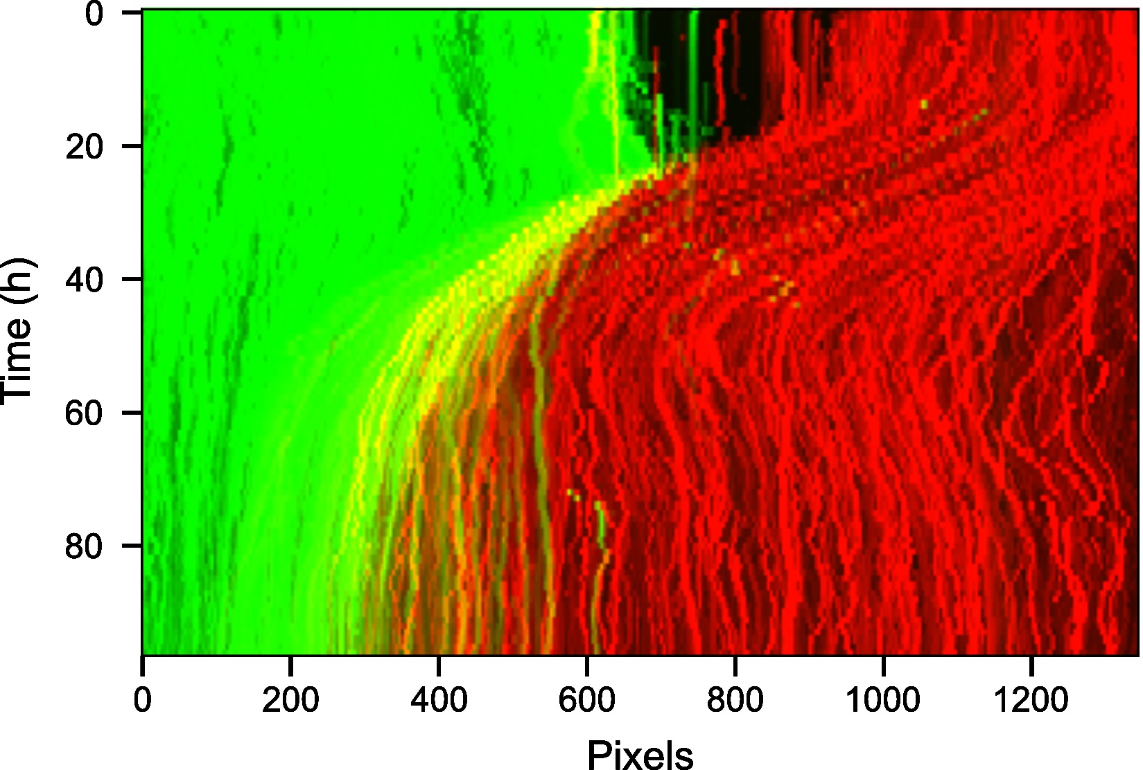
Figure 11. Kymograph of the video highlighting movement of the wound through time. The spatial row dimension of the 2D video was collapsed by using the maximum intensity along each pixel column.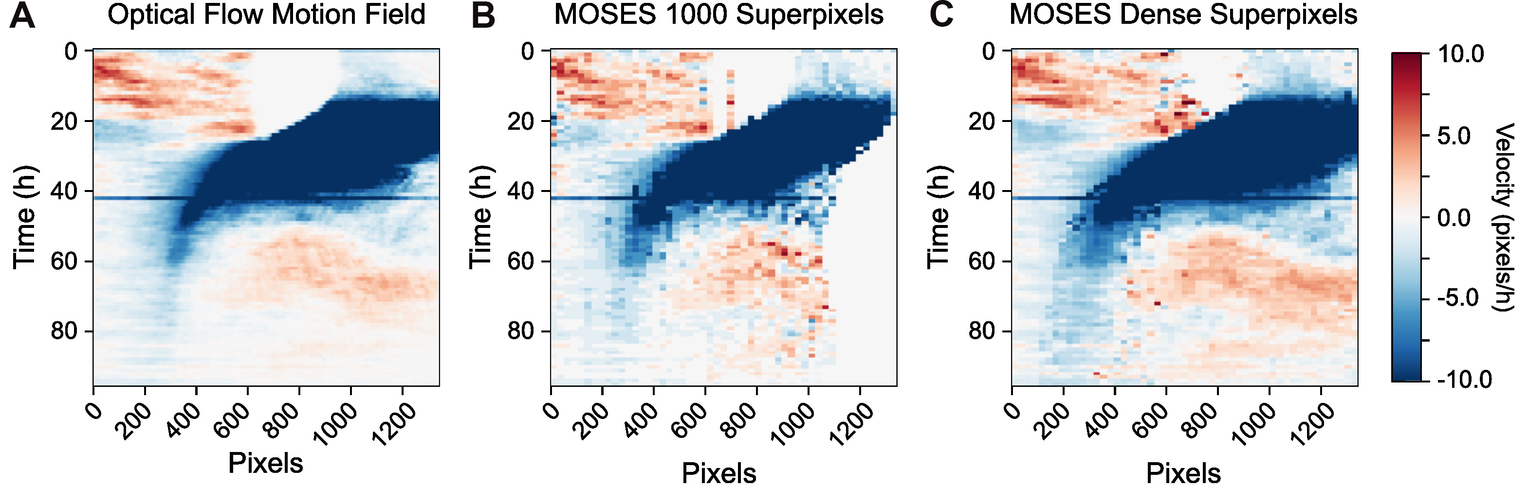
Figure 12. Velocity kymographs summarising the velocity with distance away from the interface. The velocity kymograph computed taking the median of column values of the pixel motion field (A), the superpixel tracks from tracking a fixed number of 1,000 superpixels (B) and when dense superpixel tracking is used (C).
- Compute the velocity kymograph of the pixel motion field (Figure 12A).
- Locate the interface boundary line frame to frame using the extracted superpixel tracks and subsequently fit the line to a spline approximation to enable interpolation from the image y-coordinates (Figure 13).
from MOSES.Motion_Analysis.wound_statistics_tools import boundary_superpixel_meantracks_RGB
boundary_curves, curves_lines, curve_img,boundary_line = boundary_superpixel_meantracks_RGB(vidstack, meantracks_r,meantracks_g, movement_thresh=0.2, t_av_motion=5, robust=False, lenient=False, debug_visual=False, max_dist=1.5, y_bins=50, y_frac_thresh=0.50) - Estimate the frame of gap closure by computing the distance between the boundary between both colored sheets from image segmentation. For the example you should get wound_closure_frame = 26 (Figure 14A).
from MOSES.Motion_Analysis.wound_close_sweepline_area_segmentation import wound_sweep_area_segmentation
wound_closure_frame =wound_sweep_area_segmentation(vidstack, spixel_size, max_frame=50, n_sweeps=50, n_points_keep=1, n_clusters=2, p_als=0.001, to_plot=True)
print('predictedgap closure frame is: %d' %(wound_closure_frame))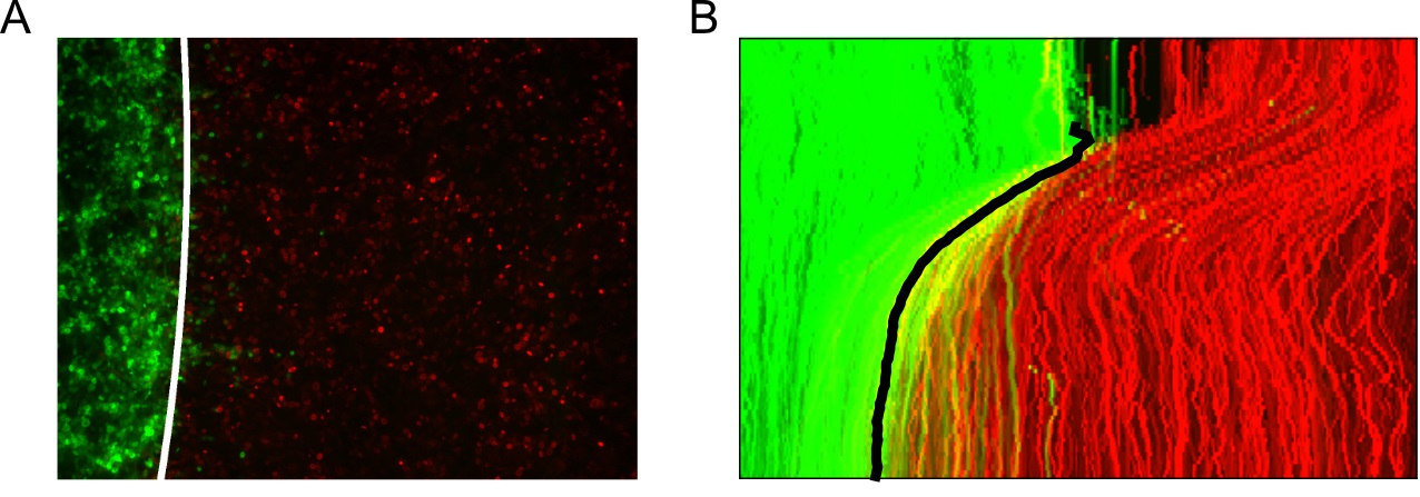
Figure 13. Tracking the interface automatically using the superpixel tracks. A. Fitted cubic spline approximation of the interface boundary plotted on the last video frame (96 h). B. Maximum intensity projection of the tracked interface boundary plotted on the video kymograph.
- Visualize the interface appearance using video kymographs. A kymograph is a projection of the 2D temporal dataset that collapses one of the spatial dimensions to allow the movement to be visualized as an image. Here the maximum along of each image pixel column was taken to summarise the motion along the image rows (Figure 11). The maximum was used to get the strongest possible signal for the interface.
- Interaction analysis
- Compute the maximum velocity cross-correlation index between red and green superpixel tracks as evidence of correlated motion of the two sheets. This measure ranges from 0 to 1 with 1 being completely correlated. For the example video, you should get a maximum velocity cross-correlation before and after gap closure of 0.022 and 0.234 suggesting increased correlation
between the movement directionality of both sheets.from MOSES.Motion_Analysis.mesh_statistics_tools import compute_max_vccf_cells_before_after_gap
(max_vccf_before, _), (max_vccf_after, _) =compute_max_vccf_cells_before_after_gap(meantracks_r, meantracks_g, wound_heal_frame=wound_closure_frame, err_frame=5)
print('max velocitycross-correlation before: %.3f' %(max_vccf_before))
print('max velocitycross-correlation after: %.3f' %(max_vccf_after)) - Compute the spatial correlation index to assess on average the extent of movement correlation between superpixel tracks and by extension cellular groups in the image. Distance is measured in normalized units as the number of superpixels away. For our video, compute the spatial correlation over a distance range of 1-6 superpixels and fit an exponential decay curve with equation, y=ae-x⁄b to extract the canonical distance, b=2.94 over which motion is correlated (Figure 14B).
Note: The computation of spatial correlation index is typically slow. Use a smaller distance range to speed up computation.from MOSES.Motion_Analysis.mesh_statistics_tools import compute_spatial_correlation_function
spatial_corr_curve,(spatial_corr_pred, a_value, b_value, r_value) =compute_spatial_correlation_function(meantracks_r, wound_closure_frame, wound_heal_err=5, dist_range=np.arange(1,6,1))
# plot thecurve and the fitted curve to y=a*exp(-x/b) to get the (a,b) parameters.
plt.figure()
plt.title('Fitted Spatial Correlation: a=%.3f, b=%.3f' %(a_value, b_value))
plt.plot(np.arange(1,6,1),spatial_corr_curve, 'ko', label='measured')
plt.plot(np.arange(1,6,1), spatial_corr_pred, 'g-', label='fitted')
plt.xlabel('Distance (Number of Superpixels)')
plt.ylabel('Spatial Correlation')
plt.legend(loc='best')
plt.show()
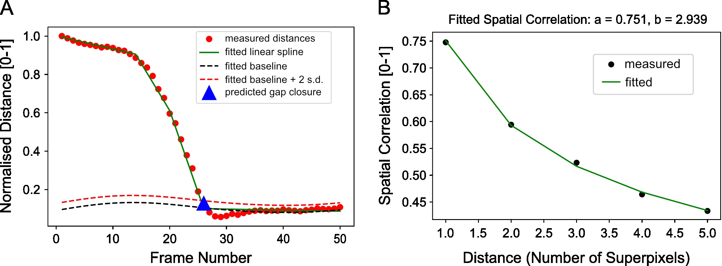
Figure 14. Example distance curve for estimating the frame of gap closure and example spatial correlation curve for estimating the distance over which cellular motion is correlated. A. Plot of the separation distance normalized by the maximum separation distance between red and green boundary points as extracted by image segmentation. Blue triangle is the final predicted gap closure frame. B. Variation of mean spatial correlation between superpixel tracks for the example video as a function of the number of superpixels away as measured by multiples of the average superpixel width. Green line is the fitted exponential decay to the black data points.
- Compute the maximum velocity cross-correlation index between red and green superpixel tracks as evidence of correlated motion of the two sheets. This measure ranges from 0 to 1 with 1 being completely correlated. For the example video, you should get a maximum velocity cross-correlation before and after gap closure of 0.022 and 0.234 suggesting increased correlation
- Motion maps
One of the primary benefits of using the superpixel tracks and meshes extracted by MOSES as discussed in our previous work (Zhou et al., 2019) was for the construction of a motion map that can be used to visually interrogate motion phenotypes. Here we describe the steps we used in the paper to construct a motion map by applying principal components analysis (PCA) to the MOSES mesh strain curve using a smaller dataset. The full datasets are available through Mendeley Datasets with DOI: https://dx.doi.org/10.17632/j8yrmntc7x.1 and https://dx.doi.org/10.17632/vrhtsdhprr.1.- Download all videos from the two folders, 0% FBS and 5% FBS folders in the Google drive (6 videos in total). They contain 3 examples each of the 0% and 5% serum cultured cell videos without EGF addition.
- Place the downloaded videos into two subfolders, 0%_FBS and 5%_FBS under a newly created top level ‘Motion_Map_Videos’ folder following the structure in Figure 1 as before.
- Automatically detect the two subfolders in the ‘Motion_Map_Videos’ folder as two separate experiment folders. The code should print a Python list with the values ['0%_FBS' '5%_FBS'].
from MOSES.Utility_Functions.file_io import detect_experiments
# detect experimentfolders as subfolders under a top-level directory.
rootfolder = '../Data/Motion_Map_Videos'
expt_folders =detect_experiments(rootfolder, exclude=['meantracks','optflow'], level1=False)
print(expt_folders) #print the detected folder names. - Use the in-built Python glob library to detect all video files using their ‘.tif’ extension in each experiment (subfolder), loading individual file paths into a single NumPy array. Subsequently create a separate integer array based on the detected files to denote if the video file came from either the ‘0%_FBS’ or ‘5%_FBS’ subfolder assigned integers ‘0’ and ‘1’ respectively.
import glob
import numpy as np
# detecteach .tif file in each folder.
videofiles =[glob.glob(os.path.join(rootfolder, expt_folder,'*.tif')) for expt_folder in expt_folders]
# shouldgive now [[0,0,0],[1,1,1]]
labels = [[i]*len(videofiles[i]) for i in range(len(videofiles))]
# flatteneverything into single array
videofiles =np.hstack(videofiles)
labels =np.hstack(labels)
- Extract superpixel tracks and compute the MOSES mesh strain curves for each video. Then concatenate the mesh strain curves of each video into one NumPy array. This constructs a feature matrix of size nsamples×dfeatures required for PCA.
Note: Augment the MOSES mesh strain curve features with image-based features such as the mean pixel intensity and texture features of the superpixel image patch to additionally describe appearance.from MOSES.Utility_Functions.file_io import read_multiimg_PIL
from MOSES.Motion_Analysis.mesh_statistics_tools import construct_MOSES_mesh, compute_MOSES_mesh_strain_curve
# set motion extractionparameters.
n_spixels = 1000
optical_flow_params = dict(pyr_scale=0.5, levels=3, winsize=15, iterations=3, poly_n=5, poly_sigma=1.2, flags=0)
n_videos = len(videofiles)
# initialise arrays tosave computed data
mesh_strain_all = []
for ii in range(n_videos):
videofile = videofiles[ii]
print(ii, videofile)
vidstack =read_multiimg_PIL(videofile)
# 1. compute superpixeltracks
_, meantracks_r = compute_grayscale_vid_superpixel_tracks(vidstack[:,:,:,0],optical_flow_params, n_spixels)
_, meantracks_g = compute_grayscale_vid_superpixel_tracks(vidstack[:,:,:,1],optical_flow_params, n_spixels)
spixel_size = meantracks_r[1,0,1] - meantracks_r[1,0,0]
# 2a. compute MOSESmesh.
MOSES_mesh_strain_time_r,MOSES_mesh_neighborlist_r = construct_MOSES_mesh(meantracks_r, dist_thresh=1.2, spixel_size=spixel_size)
MOSES_mesh_strain_time_g, MOSES_mesh_neighborlist_g= construct_MOSES_mesh(meantracks_g, dist_thresh=1.2, spixel_size=spixel_size)
# 2b. compute the MOSESmesh strain curve for the video.
mesh_strain_r =compute_MOSES_mesh_strain_curve(MOSES_mesh_strain_time_r, normalise=False)
mesh_strain_g =compute_MOSES_mesh_strain_curve(MOSES_mesh_strain_time_g, normalise=False)
mesh_strain_curve_video =.5*(mesh_strain_r+mesh_strain_g)
# (optionalnormalization)
normalised_mesh_strain_curve_video =mesh_strain_curve_video/ np.max(mesh_strain_curve_video)
# 3. append the computedmesh strain curves.
mesh_strain_all.append(normalised_mesh_strain_curve_video)
# stack all the mesh strain curves into one
mesh_strain_all = np.vstack(mesh_strain_all) - Apply PCA to the mesh strain curves of the 5% FBS videos only to set the two principal components for mapping.
Note: 0% serum videos could also have been used. Generally to learn the data variation it is recommended to use the larger dataset.from sklearn.decomposition import PCA
# initialise the PCAmodel
pca_model = PCA(n_components=2, random_state=0)
# 1. learn the PCA usingonly the 5% FBS a.k.a label=1
pca_5_percent_mesh =pca_model.fit_transform(mesh_strain_all[labels==1]) - Project the mesh strain curves of the 0% FBS videos using the principal components defined by the 5% FBS videos.
pca_0_percent_mesh =pca_model.transform(mesh_strain_all[labels==0])
- Visualize the projected PCA components on a 2D x-y axis plotting the first principal components (x-axis) vs the second principal component (y-axis) (Figure 15).
Note: The resulting PCA plot should clearly highlight the distinct separation of motion behavior between 0% FBS and 5% FBS. The exact numerical values may differ depending on installed library versions of scikit-learn, OS and random number generation settings.fig, ax = plt.subplots(figsize=(3,3))
ax.plot(pca_5_percent_mesh[:,0], pca_5_percent_mesh[:,1], 'o', ms=10, color='g', label='5% FBS')
ax.plot(pca_0_percent_mesh[:,0], pca_0_percent_mesh[:,1], 'o', ms=10, color='r', label='0% FBS')
ax.set_xlim([-2,2])
ax.set_ylim([-2,2])
plt.legend(loc='best')
plt.show()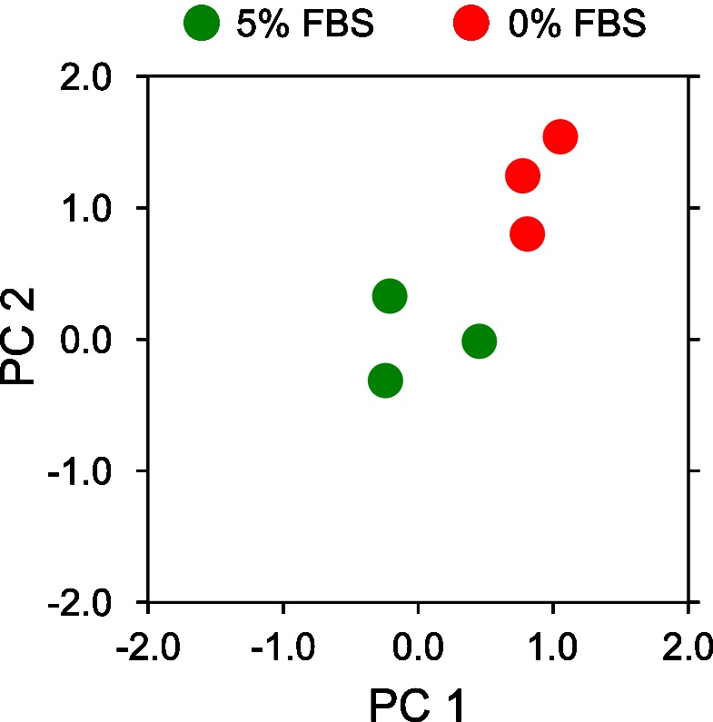
Figure 15. Motion map analysis of a reduced set of 0% and 5% serum two color epithelial cell videos
- Superpixel track cleaning for two color cell populations
Fluorescent dyes are imperfect. Despite best efforts there will often be a degree of cross-contamination across acquired color channels. This can lead to noise in the extracted motion tracks, namely green channel motion tracks may exhibit some movement when theoretically there should be none due to bleed-through from the red channel. Post-processing of the tracks can help ‘clean’ up the unspecific motion and retain only the motion of the specific superpixel tracks relevant to each initial object of interest in the respective colored channels. In doing so, one can improve the accuracy and sensitivity of analysis. One general method for cleaning is image segmentation of individual objects and retaining only the tracks that cover the segmented objects (see demo Analysis 1: Single Cell Tracking). In our paper, (Zhou et al., 2019) we instead implemented a more robust segmentation-free method that exploits motion information for colored two cell populations.- Jointly clean red and green superpixel tracks by considering the connectivity between superpixel tracks that move between the initial frame 0 and the frame specified by frame2. The resulting filtered tracks, meantracks_r_filt, meantracks_g_filt can now be used instead of meantracks_r, meantracks_g in any of the given steps for the analysis of two cell populations.
Note: Our implementation is specific for two color videos, however the principle of motion and connectivity it is based on is generalizable.from MOSES.Track_Filtering.filter_meantracks_superpixels import filter_red_green_tracks
meantracks_r_filt,meantracks_g_filt = filter_red_green_tracks(meantracks_r, meantracks_g, img_shape=(n_rows, n_cols), frame2=1)
- Jointly clean red and green superpixel tracks by considering the connectivity between superpixel tracks that move between the initial frame 0 and the frame specified by frame2. The resulting filtered tracks, meantracks_r_filt, meantracks_g_filt can now be used instead of meantracks_r, meantracks_g in any of the given steps for the analysis of two cell populations.
Analysis 3: Analysis of Drosophila Motion in Development (SiMView lightsheet Microscopy) (Supplementary files)
To demonstrate the ability of MOSES to analyze global tissue and local cellular motion patterns jointly we analyze the supplementary videos of drosophila development published by Amat et al., 2014. In addition this analysis illustrates i) how one can handle larger videos that contain a lot of temporal frames or have large video frames to speed up processing, ii) how to cluster tracks to reveal local spatial patterns and iii) how to work with general video formats such as .avi, mp4 and .mov.
- Download supplementary movie 1 (‘nmeth.3036-sv1.avi’) of Amat et al., 2014, entitled ‘SiMView imaging of Drosophila embryogenesis’.
- Construct a function to read the .avi video using the moviepy library with optional rescaling of video frame dimensions through the resize parameter. For more information using moviepy please refer to https://zulko.github.io/moviepy/.
def read_movie(moviefile, resize=1.):
from moviepy.editor import VideoFileClip
from tqdm import tqdm
from skimage.transform import rescale
import numpy as np
vidframes = []
clip = VideoFileClip(moviefile)
count = 0
for frame in tqdm(clip.iter_frames()):
vidframes.append(np.uint8(rescale(frame, 1./resize, preserve_range=True)))
count+=1
vidframes = np.array(vidframes)
return vidframes
moviefile = '../Data/Videos/nmeth.3036-sv1.avi'
# read in the movie, downsampling framesby 4.
movie = read_movie(moviefile, resize=4.)
n_frame, n_rows, n_cols, n_channels =movie.shape
print('Sizeof video: (%d,%d,%d,%d)' %(n_frame,n_rows,n_cols,n_channels)) - Set motion parameters as before and extract forward and backward superpixel tracks using dense superpixel tracking.
from MOSES.Optical_Flow_Tracking.superpixel_track import compute_grayscale_vid_superpixel_tracks_FB
# motion extractionparameters.
optical_flow_params = dict(pyr_scale=0.5, levels=5, winsize=21, iterations=5, poly_n=5, poly_sigma=1.2, flags=0)
# number of superpixels
n_spixels = 1000
# extract forward andbackward tracks.
optflow, meantracks_F, meantracks_B =compute_grayscale_vid_superpixel_tracks_FB(movie[:,:,:,1], optical_flow_params,n_spixels, dense=True)
- Cluster superpixels according to track similarity to group together similar tracks. This requires the construction of a feature matrix for each superpixel track.
- Construct the track feature, f ifor superpixel track i by concatenating the (x,y) coordinates at each time frame up to frame T such that f=[x_1,x_2,…,x_(T-1),x_T,y_1,y_2,…,y_(T-1),y_T ]. For this example, the final feature matrix, X is a matrix of 2628 x 1104.
import numpy as np
X = np.hstack([meantracks_F[:,:,0], meantracks_F[:,:,1]]) - Reduce dimensionality of feature matrix, X using principal components analysis (PCA) to compress features and improve clustering.
from sklearn.decomposition import PCA
pca_model = PCA(n_components = 3, whiten=True, random_state=0)
X_pca = pca_model.fit_transform(X) - Cluster tracks using the PCA reduced features using a Gaussian mixture model (GMM) specifying 10 clusters. The result is given as a vector array, track_labels specifying using unique integer values the group that each superpixel track has been assigned to by the GMM model. Note colors will be different for different runs of the algorithm due to randomness in the setting of the GMM algorithm.
Note: Any other clustering algorithm operating on a matrix can be used such as hierarchical clustering, K-means clustering and density based clustering.from sklearn import mixture
n_clusters = 10
gmm = mixture.GaussianMixture(n_components=n_clusters, covariance_type='full', random_state=0)
gmm.fit(X_pca)
# get the labels
track_labels = gmm.predict(X_pca)
- Construct the track feature, f ifor superpixel track i by concatenating the (x,y) coordinates at each time frame up to frame T such that f=[x_1,x_2,…,x_(T-1),x_T,y_1,y_2,…,y_(T-1),y_T ]. For this example, the final feature matrix, X is a matrix of 2628 x 1104.
- Visualize the clustered superpixel tracks coloring each unique group with a different color (Figure 16).
Note: We confirmed differences in GMM clustering results between different OS and scikit-learn library versions with the same code. The reported figure was obtained for Windows 10, scikit-
learn version 0.21.2.from MOSES.Visualisation_Tools.track_plotting import plot_tracks
import seaborn as sns
import pylab as plt
# Generate colours foreach unique cluster.
cluster_colors = sns.color_palette('hls', n_clusters)
# overlay cluster tracksand clustered superpixels
fig, ax = plt.subplots(nrows=1,ncols=3, figsize=(15,15))
ax[0].imshow(movie[0]); ax[0].grid('off');ax[0].axis('off'); ax[0].set_title('Initial Points')
ax[1].imshow(movie[-1]); ax[1].grid('off');ax[1].axis('off'); ax[1].set_title('Final Points')
ax[2].imshow(movie[0]); ax[2].grid('off');ax[2].axis('off'); ax[2].set_title('Clustered Tracks')
for ii, lab in enumerate(np.unique(track_labels)):
# plot coloured initialpoints
ax[0].plot(meantracks_F[track_labels==lab,0,1],
meantracks_F[track_labels==lab,0,0], 'o', color=cluster_colors[ii], alpha=1)
# plot coloured finalpoints
ax[1].plot(meantracks_F[track_labels==lab,-1,1],
meantracks_F[track_labels==lab,-1,0], 'o', color=cluster_colors[ii], alpha=1)
# plot coloured tracks
plot_tracks(meantracks_F[track_labels==lab],ax[2], color=cluster_colors[ii], lw=1.0, alpha=0.7)
plt.show()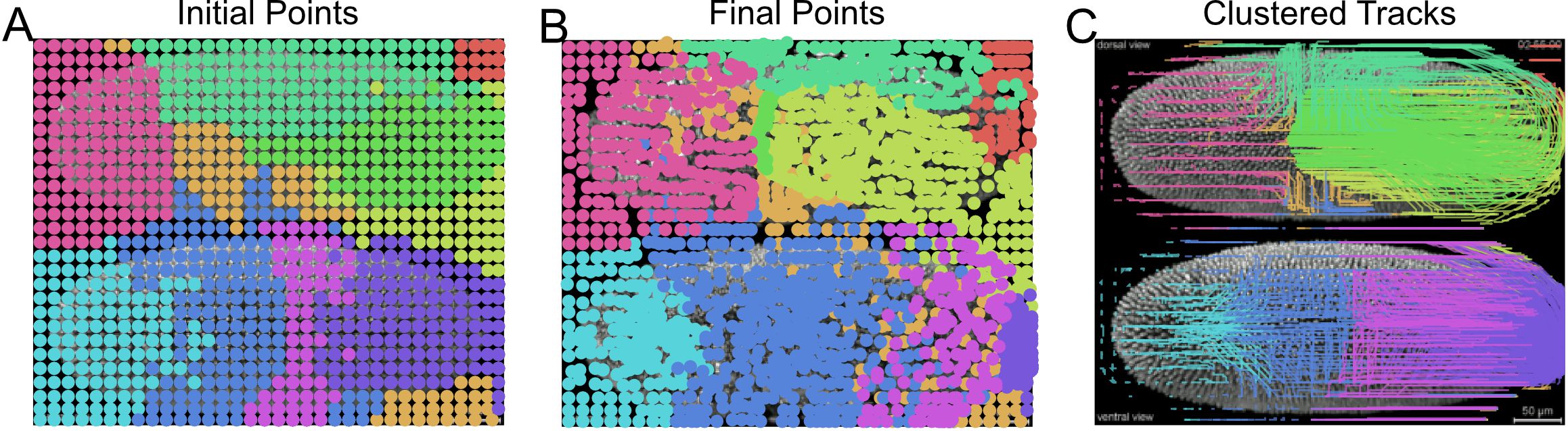
Figure 16. Unsupervised clustering of superpixel tracks to group local motion during Drosophila embryogenesis. Initial (A) and final (B) centroid positions of superpixels plotted as a dot and colored by assigned group using Gaussian mixture model for clustering. Corresponding superpixel tracks colored by cluster (C). - Compute the motion saliency map of the forward and backward tracks to find motion sources and sinks (Figure 17).
from MOSES.Motion_Analysis.mesh_statistics_tools import compute_motion_saliency_map
from skimage.exposure import equalize_hist
from skimage.filters import Gaussian
# specify a large thresholdto capture long-distances.
dist_thresh = 20
spixel_size = meantracks[1,0,1]-meantracks[1,0,0]
motion_saliency_F,motion_saliency_spatial_time_F = compute_motion_saliency_map(meantracks, dist_thresh=dist_thresh, shape=movie.shape[1:-1], max_frame=None, filt=1, filt_size=spixel_size)
motion_saliency_B,motion_saliency_spatial_time_B = compute_motion_saliency_map(meantracks_B, dist_thresh=dist_thresh, shape=movie.shape[1:-1], max_frame=None, filt=1, filt_size=spixel_size)
# smooth the discretelooking motion saliency maps.
motion_saliency_F_smooth =gaussian(motion_saliency_F, spixel_size/2.)
motion_saliency_B_smooth =gaussian(motion_saliency_B, spixel_size/2.)
# visualise the computedresults.
fig, ax = plt.subplots(nrows=1, ncols=2, figsize=(15,15))
ax[0].imshow(movie[0], cmap='gray');ax[0].grid('off'); ax[0].axis('off')
ax[1].imshow(movie[0], cmap='gray');ax[1].grid('off'); ax[1].axis('off')
ax[0].set_title('Motion Sinks');ax[1].set_title('Motion Sources')
ax[0].imshow(equalize_hist(motion_saliency_F_smooth), cmap='coolwarm', alpha=0.5, vmin=0, vmax=1)
ax[1].imshow(equalize_hist(motion_saliency_B_smooth), cmap='coolwarm', alpha=0.5, vmin=0, vmax=1)
plt.show()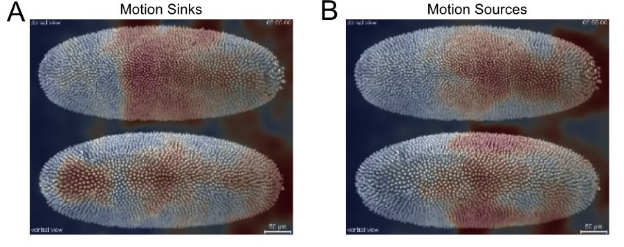
Figure 17. Motion saliency map to highlight spatial areas of motion sinks (A) and sources (B) during Drosophila embryogenesis
Analysis 4: Intra-vital Imaging Analysis (Multiphoton Microscopy) (Supplementary files)
Intra-vital imaging has enabled direct in-vivo imaging of the movement of fluorescently tagged cells in their native microenvironment. A common application is the study of immune cell behavior with respect to the local vasculature and extracellular matrix in tissue (Li et al., 2012). Typically it is desired to extract the global motion patterns of individual cell population despite their stochastic individual motion. Using automatic single-cell tracking approaches is frequently unreliable due to the lower imaging magnification and poorer spatial resolution of the acquired images compared to in-vitro imaging. For example, it is difficult for humans to manually distinguish between individually migrating fluorescent immune cells. Here we demonstrate how to use MOSES to nevertheless extract the global motion pattern of individual neutrophil cells to a laser-induced wound site for quantitative analysis.
- Download supplementary movie 1 of Li et al., 2012.
- Read the movie using the example read_movie function defined in Analysis 3 above. As the video is short and we want to retain high spatial fidelity, the native pixel resolution of image frames is used without downsampling (resize=1.).
moviefile = '../Data/Videos/nprot.2011.438-S5.mov'
movie = read_movie(moviefile, resize=1.) - Set the motion extraction parameters and extract both forward and backward superpixel tracks using 1,000 superpixels. Optionally set dense=True.
from MOSES.Optical_Flow_Tracking.superpixel_track import compute_grayscale_vid_superpixel_tracks_FB
# motion extractionparameters.
optical_flow_params = dict(pyr_scale=0.5, levels=5, winsize=21, iterations=5, poly_n=5, poly_sigma=1.2, flags=0)
# number of superpixels
n_spixels = 1000
# extract superpixeltracks for the 2nd or 'green' GFP+ cell channel
optflow, meantracks_F, meantracks_B =compute_grayscale_vid_superpixel_tracks_FB(movie[:,:,:,1], optical_flow_params,n_spixels, dense=True) - Compute the mean temporal optical flow to summarize the mean motion of image pixels over the imaged duration. Through averaging, stochastic motion is removed and globally consistent trends are reinforced. Color map the computed mean optical flow according to the directionality of motion using an HSV color scheme to visualize the average global motion pattern of GFP+ neutrophil cells (Figure 18A).
from MOSES.Visualisation_Tools.motion_field_visualisation import view_ang_flow
import numpy as np
mean_opt_flow = np.mean(optflow, axis=0)
mean_colored_flow = view_ang_flow(mean_opt_flow) - Compute the average velocity of individual superpixel tracks and the mean temporal (x,y) coordinates of superpixel tracks as the MOSES superpixel track equivalent to Step 4 above (Figure 18B).
from MOSES.Motion_Analysis.tracks_statistics_tools import average_displacement_tracks
mean_disps_tracks =average_displacement_tracks(meantracks)
# parse out the mean(u,v) velocities of tracks
U_tra = mean_disps_tracks[:,1]
# this is negative toconvert image coordinates to proper (x,y) used in matplotlib quiverplot.
V_tra = -mean_disps_tracks[:,0]
Mag_tra = np.hypot(U_tra, V_tra)
# compute the mean (x,y)position of tracks
X_mean = np.mean(meantracks[:,:,1], axis=-1)
Y_mean = np.mean(meantracks[:,:,0], axis=-1) - Compute the forward and backward motion saliency maps using the forward and backward superpixel tracks to reveal motion ‘sinks’ and ‘sources’ respectively (Figure 18B).
from MOSES.Motion_Analysis.mesh_statistics_tools import compute_motion_saliency_map
from skimage.exposure import equalize_hist
from skimage.filters import Gaussian
# specify a largethreshold to capture long-distances.
dist_thresh = 5
spixel_size = meantracks[1,0,1]-meantracks[1,0,0]
# compute the forwardand backward motion saliency maps.
motion_saliency_F,motion_saliency_spatial_time_F = compute_motion_saliency_map(meantracks, dist_thresh=dist_thresh, shape=movie.shape[1:-1], max_frame=None, filt=1, filt_size=spixel_size)
motion_saliency_B,motion_saliency_spatial_time_B = compute_motion_saliency_map(meantracks_B, dist_thresh=dist_thresh, shape=movie.shape[1:-1], max_frame=None, filt=1, filt_size=spixel_size)
# smooth the discretelooking motion saliency maps.
motion_saliency_F_smooth =gaussian(motion_saliency_F, spixel_size/2.)
motion_saliency_B_smooth =gaussian(motion_saliency_B, spixel_size/2.)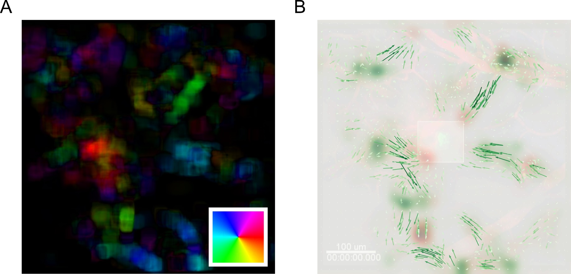
Figure 18. MOSES analysis unbiasedly uncovers the migration of GFP+ neutrophil cells to site of laser injury. A. Mean motion field after averaging over all time points. Direction of motion is colored according to the inset color wheel. Colour intensity represents the magnitude of the velocity. B. Overlay of the mean superpixel track velocities represented as green arrows plotted on top of the first video frame. Additionally, the computed forward and backward motion saliency maps are shown as red and green heatmaps revealing local motion sinks and sources respectively. Square box in the middle indicates the induced laser injury site.
Notes
We highlight key common considerations that arise when conducting a MOSES analysis to extract superpixel tracks, computing the motion saliency map and constructing motion maps. In general, MOSES is reproducible, produces consistent and interpretable results for all types of imaging as long as its primary modeling assumptions are satisfied.
- Key analysis assumptions of MOSES–two general key principles govern the behavior and accuracy of MOSES
- MOSES implicitly assumes that the motion of interest is the most dominant contributor of motion in the video. This is the most important assumption of MOSES. Given a video many factors may influence the motion of the image pixels for example camera movement and stage movement cause global shifts in the field of view and cell division induce local motion. MOSES does not explicitly disentangle the contribution to the global measured motion from different sources. If multiple sources of motion are present with similar magnitudes such as the deformation of the extra-cellular matrix and cellular migration in intra-vital images, non-rigid image registration should be applied first to remove the extra-cellular deformations before running MOSES to analyze only the cellular motion component.
- MOSES superpixel tracks extract the movement trajectory that follows the most dominant local motion pattern. Individual superpixels are updated through time according to the average (mean or median) velocity of individual pixels within it. Should bimodality exist in the local directionality, MOSES would update the superpixel position according to the more dominant direction. This may cause the superpixels to no longer follow the same moving entity. Thus single MOSES tracks are not guaranteed to follow any individual cell or cell group however the extraction of dominant global and local motion patterns and the analysis of motion source and sinks becomes very natural. Given no restriction on the movement of superpixels as they are updated over time, should dominant local motion patterns exist then they will naturally aggregate together surrounding superpixels and statistically upvote these image regions. By exploiting these phenomena, the salient motion patterns within a video can be efficiently and unbiasedly uncovered and encoded into ‘signatures’ for phenotyping.
- MOSES implicitly assumes that the motion of interest is the most dominant contributor of motion in the video. This is the most important assumption of MOSES. Given a video many factors may influence the motion of the image pixels for example camera movement and stage movement cause global shifts in the field of view and cell division induce local motion. MOSES does not explicitly disentangle the contribution to the global measured motion from different sources. If multiple sources of motion are present with similar magnitudes such as the deformation of the extra-cellular matrix and cellular migration in intra-vital images, non-rigid image registration should be applied first to remove the extra-cellular deformations before running MOSES to analyze only the cellular motion component.
- Setting the number of superpixels
The number of superpixels directly determines the size of the region of interest (ROI) being tracked. Less superpixels or larger ROI capture coarse motion patterns that affect larger areas but lose resolution in the motion information due to computing the average over a larger spatial area. Conversely more superpixels or smaller ROI better capture finer motion patterns but velocities may be more subject to outliers. Finally, there is a speed consideration. More superpixels take longer to track. Typically the number of superpixels used should be the minimum necessary to capture the spatial scale of the desired motion pattern. As a guide start with 1,000 superpixels. If too fine try 100 superpixels, if too coarse try 10,000 superpixels. - Setting the optical flow motion extraction parameters
Optical flow algorithms aim to estimate the local motion field by finding the optimal set of displacements (Δx,Δy) that minimize the difference of the pixel intensities between two frames separated by a small time Δt. Mathematically this solves for the following equality
I(x,y,t)=I(x+Δx,y+Δy,t+Δt)
where I(x,y,t) is the pixel intensity values of the video frame at time t. The OpenCV Farnebäck optical flow algorithm used in MOSES solves this problem using local image patches of a fixed user-specified size similar to particle image velocimetry. To capture larger displacements than the fixed window size (given by the number of pixels), the original image is first downsampled and smoothed multiple times resulting in an image pyramid. The optimization problem is then solved progressively starting from the lowest level of the image pyramid with the most downsampled image and ending at the topmost level of the image pyramid, the original image to yield the final set of displacements. In this manner, the same fixed window size in lower pyramid levels corresponds to increasingly larger areas at the original image scale. The main consideration when setting the parameters for optical flow estimation is choosing a set of parameters that best captures any long, discontinuous displacements between successive video frames. This type of motion is very common for particle-like objects and cells undergoing single-cell motion. To better capture large, discontinuous displacements one can increase the window size (winsize), increase the number of levels in the pyramid (levels) or decrease the scaling factor (pyr_scale) to create smaller images per pyramid level. Note the number of pyramid levels and pyramid scale is related as the upper limit of the number of pyramid levels is bounded by the original image size and the scaling factor. In practice changing the number of levels is easier to tune. The optimization process is iterative thus increasing the number of iterations leads to more accurate results. Adjustment of these parameters typically requires longer computation times per video frame. We recommended starting parameters of pyr_scale=0.5, levels=3, winsize=15, iterations=3 for confluent cell motion similar to those in epithelial sheets. - Rescaling image intensity before optical flow extraction
It is important to rescale image intensities prior to motion extraction with optical flow. Ideally all video frames should be of the same brightness and well contrasted. If this is not the case it is recommended to rescale the image intensities of each video frame to their respective minimum and maximum values. Alternatively one can correct for the brightness variation using a known mathematical model for example an exponential decay model for fluorescence microscopy. - Setting the distance threshold in the mesh construction and motion saliency map computation
Similar to the number of superpixels, the distance threshold should be set according to the spatial range of the phenomena to be captured. Larger distance thresholds capture more neighboring superpixel tracks and give more information regarding events that act on longer spatial scales such as boundary formation. Conversely smaller distance thresholds are more useful when considering phenomena that occur over a very localized region such as neutrophil migration to local wound sites. We recommend experimenting with different values for the distance threshold. It should be noted that results are generally stable over a wide range of distance thresholds. - Feature construction for use in motion map construction
The interested reader should refer to the supplementary information of the original MOSES paper (Zhou et al., 2019) where we discussed in detail how to construct informative features for more general datasets. In brief, there is no one method fits all approach. Users should construct a set of features that best capture the appearance and movement variation exhibited by moving entities in the video. For epithelial sheets where individual cell morphology is not readily visible, the use of only motion-based features like the proposed mesh strain curve should be sufficient. For sparsely plated single cells that exhibit morphological changes over time, the incorporation of appearance features is also important. For large datasets, one might consider training deep learning feature extractors. The more informative the features used, the less sophisticated the algorithm required for projecting the features when constructing a 2D or 3D motion map.
Acknowledgments
This work is an accompaniment to our original methods paper published in eLife (Zhou et al., 2019) and extends the original work to showcase more the practical use of MOSES on a wide variety of imaging datasets. We thank Prof. Hiroshi Nakagawa for the generous donation of EPC2 cells originally used in the study of Harada et al., 2013. We thank Mark Shipman for technical assistance with timelapse microscopy in the collection of the two cell population dataset. This work was mainly funded by the Ludwig Institute for Cancer Research (LICR) with additional support from a CRUK grant to XL (C9720/A18513). FYZ is funded through the EPSRC Life Sciences Interface Doctoral Training Centre EP/F500394/1 and LICR, CRP and XL are funded by LICR, RPO is supported by LICR, the Oxford Health Services Research Committee and Oxford University Clinical Academic Graduate School supported by the National Institute for Health Research (NIHR) Biomedical Research Centre based at the Oxford University Hospitals Trust, Oxford, MJW is supported by CRUK (C5255/A19498, through an Oxford Cancer Research Centre Clinical Research Training Fellowship), and JR is funded by LICR and the EPSRC SeeBiByte Programme Grant (EP/M013774/1). The views expressed herein are those of the authors and not necessarily those of the NHS, the NIHR or the Department of Health.
Competing interests
A patent is pending for MOSES (UK application no. GB1716893.1, International application no. PCT/GB2018/052935). MOSES is available open-source and free for all academic and non-profit users under a Ludwig academic and non-profit license.
References
- Amat, F., Lemon, W., Mossing, D. P., McDole, K., Wan, Y., Branson, K., Myers, E. W. and Keller, P. J. (2014). Fast, accurate reconstruction of cell lineages from large-scale fluorescence microscopy data. Nat Methods 11(9): 951-958.
- Farnebäck, G. (2003). Two-frame motion estimation based on polynomial expansion. In: Bigun, J. and Gustavsson, T. (Eds.). Image Analysis. SCIA 2003. Lecture Notes in Computer Science, vol 2749. Springer, Berlin, Heidelberg.
- Harada, H., Nakagawa, H., Oyama, K., Takaoka, M., Andl, C.D., Jacobmeier, B., von Werder, A., Enders, G.H., Opitz, O.G. and Rustgi, A.K. (2003). Telomerase induces immortalization of human esophageal keratinocytes without p16INK4a inactivation. Molecular Cancer Research, 1(10): 729-738.
- Li, J. L., Goh, C. C., Keeble, J. L., Qin, J. S., Roediger, B., Jain, R., Wang, Y., Chew, W. K., Weninger, W. and Ng, L. G. (2012). Intravital multiphoton imaging of immune responses in the mouse ear skin. Nat Protoc 7(2): 221-234.
- Maška, M., Ulman, V., Svoboda, D., Matula, P., Matula, P., Ederra, C., Urbiola, A., Espana, T., Venkatesan, S., Balak, D. M., Karas, P., Bolckova, T., Streitova, M., Carthel, C., Coraluppi, S., Harder, N., Rohr, K., Magnusson, K. E., Jalden, J., Blau, H. M., Dzyubachyk, O., Krizek, P., Hagen, G. M., Pastor-Escuredo, D., Jimenez-Carretero, D., Ledesma-Carbayo, M. J., Munoz-Barrutia, A., Meijering, E., Kozubek, M. and Ortiz-de-Solorzano, C. (2014). A benchmark for comparison of cell tracking algorithms. Bioinformatics 30(11): 1609-1617.
- Meijering, E., Dzyubachyk, O. and Smal, I. (2012). Methods for cell and particle tracking. Methods Enzymol 504: 183-200.
- Milde, F., Franco, D., Ferrari, A., Kurtcuoglu, V., Poulikakos, D. and Koumoutsakos, P. (2012). Cell Image Velocimetry (CIV): boosting the automated quantification of cell migration in wound healing assays. Integr Biol (Camb) 4(11): 1437-1447.
- Neumann, B., Held, M., Liebel, U., Erfle, H., Rogers, P., Pepperkok, R. and Ellenberg, J. (2006). High-throughput RNAi screening by time-lapse imaging of live human cells. Nat Methods 3(5): 385-390.
- Nketia, T. A., Sailem, H., Rohde, G., Machiraju, R. and Rittscher, J. (2017). Analysis of live cell images: Methods, tools and opportunities. Methods 115: 65-79.
- Padfield, D., Rittscher, J. and Roysam, B. (2011). Coupled minimum-cost flow cell tracking for high-throughput quantitative analysis. Med Image Anal 15(4): 650-668.
- Petitjean, L., Reffay, M., Grasland-Mongrain, E., Poujade, M., Ladoux, B., Buguin, A. and Silberzan, P. (2010). Velocity fields in a collectively migrating epithelium. Biophys J 98(9): 1790-1800.
- Schiegg, M., Hanslovsky, P., Haubold, C., Koethe, U., Hufnagel, L. and Hamprecht, F. A. (2015). Graphical model for joint segmentation and tracking of multiple dividing cells. Bioinformatics 31(6): 948-956.
- Szabó, B., Szöllösi, G. J., Gönci, B., Jurányi, Z., Selmeczi, D. and Vicsek, T. (2006). Phase transition in the collective migration of tissue cells: experiment and model. Phys Rev E Stat Nonlin Soft Matter Phys 74(6 Pt 1): 061908.
- Zaritsky, A., Natan, S., Ben-Jacob, E. and Tsarfaty, I. (2012). Emergence of HGF/SF-induced coordinated cellular motility. PLoS One 7(9): e44671.
- Zaritsky, A., Kaplan, D., Hecht, I., Natan, S., Wolf, L., Gov, N. S., Ben-Jacob, E. and Tsarfaty, I. (2014). Propagating waves of directionality and coordination orchestrate collective cell migration. PLoS Comput Biol 10(7): e1003747.
- Zaritsky, A., Welf, E. S., Tseng, Y. Y., Angeles Rabadan, M., Serra-Picamal, X., Trepat, X. and Danuser, G. (2015). Seeds of locally aligned motion and stress coordinate a collective cell migration. Biophys J 109(12): 2492-2500.
- Zaritsky, A., Tseng, Y. Y., Rabadan, M. A., Krishna, S., Overholtzer, M., Danuser, G. and Hall, A. (2017). Diverse roles of guanine nucleotide exchange factors in regulating collective cell migration. J Cell Biol 216(6): 1543-1556.
- Zhou, F. Y., Ruiz-Puig, C., Owen, R. P., White, M. J., Rittscher, J. and Lu, X. (2019). Motion sensing superpixels (MOSES) is a systematic computational framework to quantify and discover cellular motion phenotypes. Elife 8: pii: e40162.
文章信息
版权信息
![]() Zhou et al. This article is distributed under the terms of the Creative Commons Attribution License (CC BY 4.0).
Zhou et al. This article is distributed under the terms of the Creative Commons Attribution License (CC BY 4.0).
如何引用
Readers should cite both the Bio-protocol article and the original research article where this protocol was used:
- Zhou, F. Y., Ruiz-Puig, C., Owen, R. P., White, M. J., Rittscher, J. and Lu, X. (2019). Characterization of Biological Motion Using Motion Sensing Superpixels. Bio-protocol 9(18): e3365. DOI: 10.21769/BioProtoc.3365.
- Zhou, F. Y., Ruiz-Puig, C., Owen, R. P., White, M. J., Rittscher, J. and Lu, X. (2019). Motion sensing superpixels (MOSES) is a systematic computational framework to quantify and discover cellular motion phenotypes. Elife 8: pii: e40162.
分类
细胞生物学 > 细胞成像 > 活细胞成像
细胞生物学 > 组织分析 > 组织成像
您对这篇实验方法有问题吗?
在此处发布您的问题,我们将邀请本文作者来回答。同时,我们会将您的问题发布到Bio-protocol Exchange,以便寻求社区成员的帮助。