- Protocols

- Articles and Issues
- For Authors
- About
- Become a Reviewer

Modeling the Nonlinear Dynamics of Intracellular Signaling Networks
Published: Vol 11, Iss 14, Jul 20, 2021 DOI: 10.21769/BioProtoc.4089 Views: 4108
Reviewed by: Chiara AmbrogioPablo Bolanos-VillegasAnonymous reviewer(s)
Original research article
The authors used this protocol in:

Jul 2020
Advertisement


Protocol Collections
Comprehensive collections of detailed, peer-reviewed protocols focusing on specific topics


Abstract
This protocol illustrates a pipeline for modeling the nonlinear behavior of intracellular signaling pathways. At fixed spatial points, nonlinear signaling dynamics are described by ordinary differential equations (ODEs). At constant parameters, these ODEs may have multiple attractors, such as multiple steady states or limit cycles. Standard optimization procedures fine-tune the parameters for the system trajectories localized within the basin of attraction of only one attractor, usually a stable steady state. The suggested protocol samples the parameter space and captures the overall dynamic behavior by analyzing the number and stability of steady states and the shapes of the assembly of nullclines, which are determined as projections of quasi-steady-state trajectories into different 2D spaces of system variables. Our pipeline allows identifying main qualitative features of the model behavior, perform bifurcation analysis, and determine the borders separating the different dynamical regimes within the assembly of 2D parametric planes. Partial differential equation (PDE) systems describing the nonlinear spatiotemporal behavior are derived by coupling fixed point dynamics with species diffusion.
Keywords: Cell signalingBackground
Here, we present a protocol for computational analysis of the nonlinear dynamic behavior of signaling networks and their transitions between different dynamic regimes. The dynamics of spatially homogenous biochemical systems are described by ordinary differential equations (ODE), whereas the spatiotemporal dynamics are described by partial differential equation (PDE) systems. Knowledge about ODE and PDE is needed as a prerequisite for understanding this protocol. Our computational protocol analyzes the systems’ dynamics at fixed spatial points, and it considers the nonlinear spatiotemporal behavior by coupling fixed point dynamics with species diffusion (Tsyganov et al., 2012; Bolado-Carrancio et al., 2020). A variable xi that is the concentration or activity of each network node i depends on the time (t) in an ODE system and on both the time and the spatial coordinates in a PDE system. The described protocol operates with the already established interaction topology of the signaling network under study; that is, for each node i it is known what nodes activate and/or inhibit it. Mathematically, the network topology is determined by the signed incidence matrix of the ODE system,

If node j activates or inhibits node i (∂fi/∂xj>0 or ∂fi/∂xj,<0, respectively), the element (i,j)of the signed incidence matrix equals 1 or -1, respectively, and it equals zero if node j does not affect node i.
Traditional modeling pipelines for ODE systems use parameter optimization procedures, which rely on the fitting of simulated trajectories to experimental data points, and then study the behavior of a calibrated model (Glover et al., 2000; Maiwald and Timmer, 2008; Kreutz and Timmer, 2009; Penas et al., 2015; Thomas et al., 2016; Degasperi et al., 2017; Mitra et al., 2018 and 2019). These pipelines produce satisfactory results when the system under study has a single stable steady state or when the system trajectories are within the basin of attraction of a stable steady state for bistable or multistable biochemical systems. Recently, parameter optimization procedures have been applied to calibrate oscillatory processes and to search for oscillatory and bistable mass-action networks (Pitt and Banga, 2019; Porubsky and Sauro, 2019). However, for biological systems with multiple attractors – such as steady-state focus nodes, limit cycles, or more complex chaotic structures, which can co-exist at the same parameter values – the use of standard parameter optimization pipelines that fit time-series data might be extremely challenging. Also, systems of higher than 2D dimensions can potentially exhibit chaotic dynamics, typically happening according to one of the following scenarios: (i) period-doubling bifurcations, (ii) a transition to chaos through intermittency, and (iii) chaotization of quasi-periodic dynamics (i.e., through the destruction of multidimensional tori) (Argyris et al., 1993; Kuznetsov, 2012).
Key aspects of the behavior of 2D dynamic systems are determined by the shapes of the nullclines (Tsyganov et al., 2012). Likewise, when a high-dimensional system does not exhibit the chaotic behavior, the assembly of nullclines that are projections of quasi-steady-state (QSS) trajectories into different 2D spaces help us understand the intricate system dynamics. To obtain the QSS trajectories, we change only one variable, whereas all other variables became implicit functions of that variable. Parameter optimization software packages developed for systems biology do not operate with nullclines. A critical feature of our computational pipeline is a combination of intensive sampling of the parameters space, identification of the number and stability of steady states, and the calculation and analysis of nullclines. Only when the key properties of nullclines are determined, the standard fitting software [e.g., BioNetFit (Thomas et al., 2016; Mitra et al., 2019) or PEPSSBI (Degasperi et al., 2017)] is used for fine-tuning of the parameters. After the dynamic regimes of the reduced 2D systems are established, the behavior of the original, high-dimensional system is investigated in the vicinity of attractors found for reduced systems. This pipeline allows developing predictive models of such systems in a semi-automatic regime.
A schematic diagram highlighting the main steps of the proposed protocol is shown in Figure 1. The process consists of five successive stages:
1. Build an ODE model of the signaling network and constrain the parameter ranges using the available data on the protein abundances and kinetic constants.
2. Using a software package, e.g., the DYVIPAC package (Nguyen et al., 2015), which uses the libroadrunner library (Somogyi et al., 2015) for importing and solving ODE models, sample the parameter space, determine the number and stability of steady states for a given set of parameters, and analyze the shapes of nullclines by projecting the QSS trajectories into different 2D planes.
3. Scan 2D parametric planes and determine the types of bifurcations that occur in the system.
4. If for given dynamic regimes the system trajectories are measured, fine-tune the parameters to minimize deviations of simulated trajectories from the measured time series data using local search algorithms [e.g., simplex from BioNetFit package (Mitra et al., 2019)].
5. Based on the established dynamic regimes that often differ in distinct spatial regions, formulate a PDE system and perform spatial calculations.
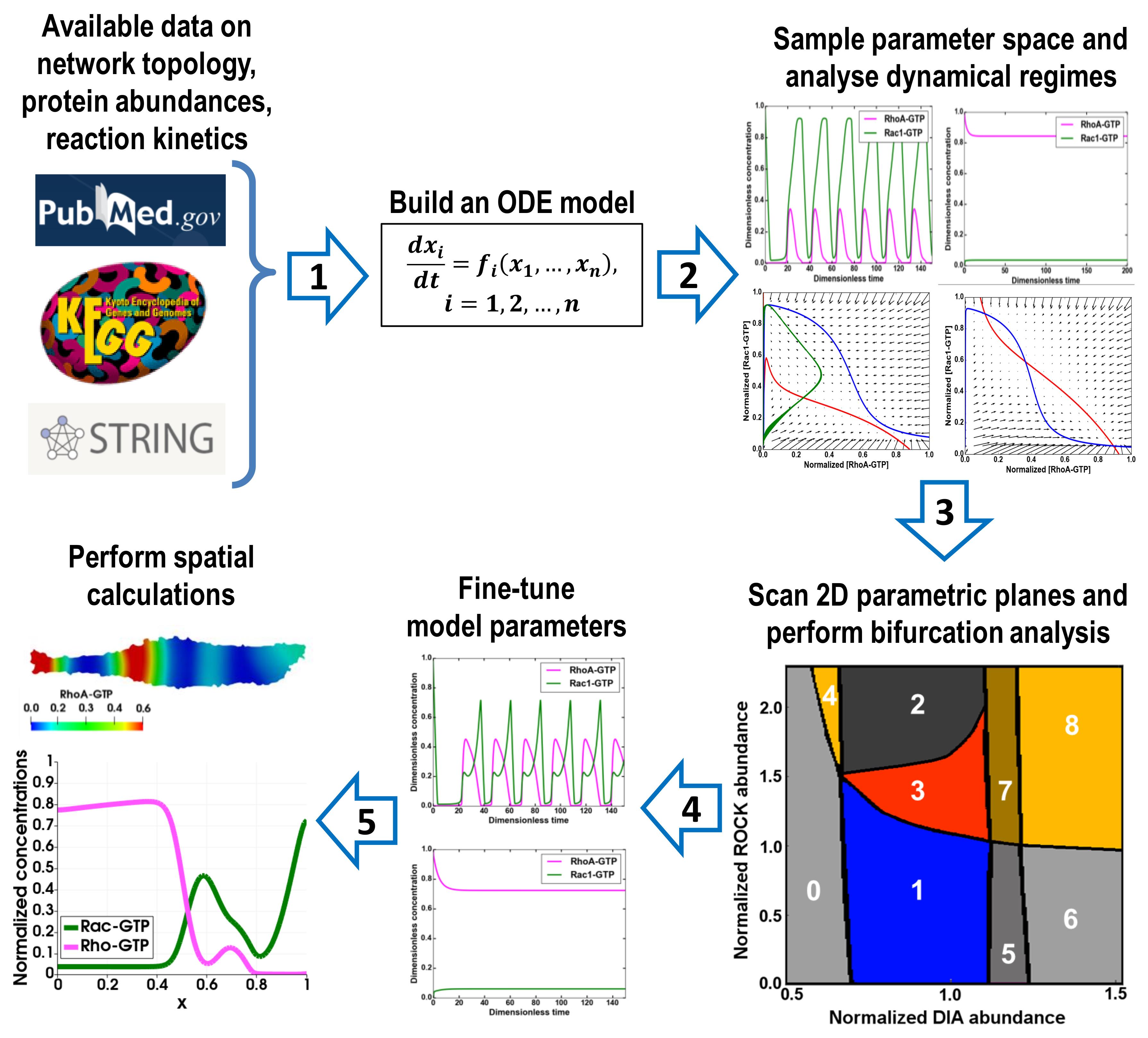
Figure 1. Protocol overview. Consecutive steps of the protocol are indicated by arrows.
Equipment
Laptop computer
Proposed protocols can be implemented on a laptop computer; however, parameter sampling procedure is time-consuming, and using a computational cluster is advantageous. For example, sampling parameter space of the model (Bolado-Carrancio et al., 2020) to obtain a comprehensive list of different regimes took approximately 5 days at a workstation with 4-core Intel® CoreTM i7 Processor. The high-quality scan of 2D parametric plane takes approximately 5 hours given the same computational power. Because the sampling procedures are very well parallelized, the computational time is inversely proportional to the number of available cores.
Since most computational clusters use Linux-based operating systems, we further refer to software packages mainly developed for Linux.
Software
Python and python libraries, including matplotlib (Hunter, 2007), NumPy (Harris et al., 2020), and scipy (Virtanen et al., 2020)
Python version of DYVIPAC software package (Nguyen et al., 2015)
Software for parameter fitting of ODE systems, e.g., BioNetFit (Thomas et al., 2016; Mitra et al., 2019), PEPSSBI (Degasperi et al., 2017), etc.
Software for performing spatiotemporal calculations of reaction-diffusion-convection models, e.g., FiPy (Guyer et al., 2009), OpenFOAM (Jasak, 2009; OpenCFD, 2009) or Virtual Cell (Loew and Schaff, 2001)
Procedure
Build an ODE model of the signaling network based on the available topology of interactions between nodes. Implement the model in a software package that supports export to the SBML format, such as COPASI (Hoops et al., 2006) or BioNetGen (Blinov et al., 2004; Harris et al., 2016).
If the kinetics of interactions between two nodes is known, this network connection is modeled mechanistically.
For other connections, the interaction kinetics might not yet be exact mechanistically characterized, or these connections operate via intermediate species that are not included in the network under study. These connections are modeled using hyperbolic multipliers αij that specify the negative or positive influence of the activity (xj) of node j on the activity (xi) of node i (Tsyganov et al., 2012; Bolado-Carrancio et al., 2020),

The coefficient γij>1 indicates activation; γij<1 inhibition; and γij=1 denotes the absence of regulatory interactions, in which case the modifying multiplier αij equals 1. Kij is the activation or inhibition constant.
Specify the parameter ranges using the data on the protein abundances and kinetic constants and assign numerical values to model parameters.
Non-dimensionalize the model to reduce the number of parameters (Barenblatt, 2003).
Export the model to SBML format.
Determine dynamical regimes that can be observed in the system.
Import the sbml-file of the model into the DYVIPAC package. Sample parameter space of the model using the DYVIPAC package, which determines the number and stability of steady states for a given set of parameters.
Rank protein abundances in a model in descending order and pick two proteins (nodes) with the highest abundance. Using the QSS approximation for the other protein activities (Sauro and Kholodenko, 2004; Eilertsen and Schnell, 2020), derive a 2D model from the initial ODE model.
Based on the specification of the steady states and the analysis of the shapes of nullclines (Figure 2, for example), determine the dynamic regimes and validate these regimes by the integration of ODEs.
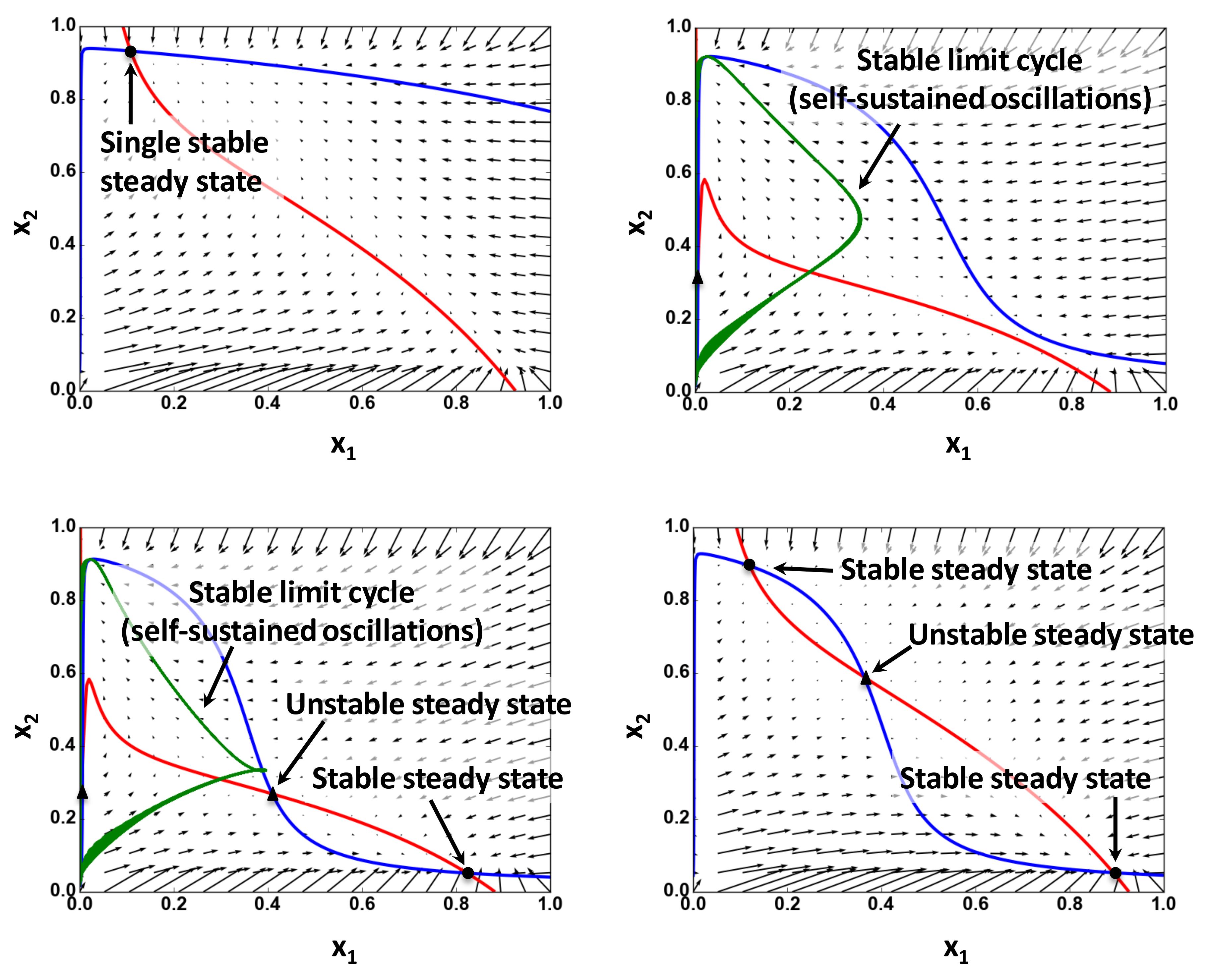
Figure 2. Examples of the nullcline analysis. Nullclines and vector fields calculated for 2D ODE system are derived from a five-dimensional ODE system using a quasi-steady-state approximation. Circles show stable steady states; triangles represent unstable steady states. Red and blue curves are nullclines for variables x1 and x2, respectively. Green line represents trajectories of limit cycles projected from the original five-dimensional system to 2D space of x1 and x2 [see Bolado-Carrancio et al. (2020) for details].If more than two proteins have high and comparable abundances, make a list of pairs of these proteins and apply the above point c) to the ODE system for each pair.
Scan 2D parametric planes and determine the types of bifurcations that can occur in the system.
Scan the parameter planes and determine the borders that separate different dynamic regimes (see Figure 3, for example). This step can predict the previously unobserved dynamic regimes, which must be validated in the experiments.
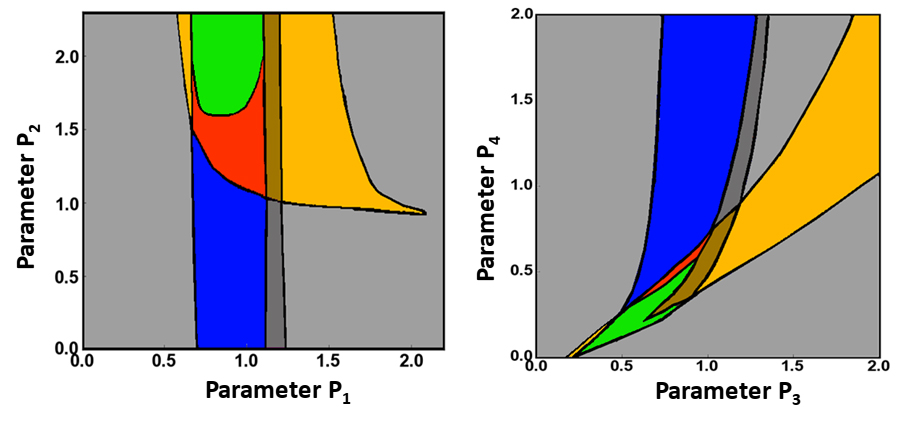
Figure 3. Examples of 2D parametric scans. Different 2D parametric diagrams obtained using scanning of 2-parameter planes. Different colors indicate different dynamical regimes. Black lines represent borders between these regimes where bifurcations happen (see Bolado-Carrancio et al., 2020 for details and Figure 2 there).The analysis of the changes in the number and stability of steady states can reveal local bifurcations, such as the Andronov-Hopf or saddle-node bifurcations (Kuznetsov, 2004). However, non-local bifurcations might exist in a 2D system where a limit cycle can appear or vanish (Nekorkin, 2015). Scan the parameters for dynamic regimes that contain focuses to determine the appearance or annihilation of limit cycles.
If there are time-series data, fine-tune model parameters to reproduce the system trajectories for a biologically relevant regime. This step uses standard software packages for parameter optimization (Glover et al., 2000; Maiwald and Timmer, 2008; Kreutz and Timmer, 2009; Penas et al., 2015; Thomas et al., 2016; Degasperi et al., 2017; Mitra et al., 2018 and 2019).
Derive a PDE system by adding the terms describing mass transfer processes such as diffusion and convection to the ODE system studied (Tsyganov et al., 2012; Bolado-Carrancio et al., 2020). Perform spatiotemporal simulations using specific software packages, such as OpenFOAM, FiPy, or Virtual Cell.
A set of examples that illustrate the analysis of the dynamics of the RhoA-Rac1 signaling network model and python scripts can be found in “examples.zip” archive.
Acknowledgments
This protocol was adapted from Tsyganov et al. (2012) and Bolado-carrancio et al. (2020). This work was supported by NIH/NCI grant R01CA244660 and EU grant NanoCommons (grant no. 731032).
Competing interests
The authors declare no competing interests.
References
- Argyris, J., Faust, G., and Haase, M. (1993). Routes to Chaos and Turbulence. A Computational Introduction. In: Philosophical Transactions of the Royal Society of London. Series A: Physical and Engineering Sciences 344: 207-234.
- Barenblatt, G. I. (2003). Scaling. Cambridge University Press, Cambridge.
- Blinov, M. L., Faeder, J. R., Goldstein, B. and Hlavacek, W. S. (2004). BioNetGen: software for rule-based modeling of signal transduction based on the interactions of molecular domains. Bioinformatics 20(17): 3289-3291.
- Bolado-Carrancio, A., Rukhlenko, O. S., Nikonova, E., Tsyganov, M. A., Wheeler, A., Garcia-Munoz, A., Kolch, W., von Kriegsheim, A. and Kholodenko, B. N. (2020). Periodic propagating waves coordinate RhoGTPase network dynamics at the leading and trailing edges during cell migration. Elife 9: e58165.
- Degasperi, A., Fey, D. and Kholodenko, B. N. (2017). Performance of objective functions and optimisation procedures for parameter estimation in system biology models. NPJ Syst Biol Appl 3: 20.
- Eilertsen, J. and Schnell, S. (2020). The quasi-steady-state approximations revisited: Timescales, small parameters, singularities, and normal forms in enzyme kinetics. Math Biosci 325: 108339.
- Glover, F., Laguna, M. and Martí, R. (2000). Fundamentals of scatter search and path relinking. Control and Cybernetics 29: 652-684.
- Guyer, J.E., Wheeler, D. and Warren, J. A. (2009). FiPy: Partial Differential Equations with Python. Comput Sci Eng 11(3): 6-15.
- Harris, C. R., Millman, K. J., van der Walt, S. J., Gommers, R., Virtanen, P., Cournapeau, D., Wieser, E., Taylor, J., Berg, S., Smith, N. J., Kern, R., Picus, M., Hoyer, S., van Kerkwijk, M. H., Brett, M., Haldane, A., Del Rio, J. F., Wiebe, M., Peterson, P., Gerard-Marchant, P., Sheppard, K., Reddy, T., Weckesser, W., Abbasi, H., Gohlke, C. and Oliphant, T. E. (2020). Array programming with NumPy. Nature 585(7825): 357-362.
- Harris, L. A., Hogg, J. S., Tapia, J. J., Sekar, J. A., Gupta, S., Korsunsky, I., Arora, A., Barua, D., Sheehan, R. P. and Faeder, J. R. (2016). BioNetGen 2.2: advances in rule-based modeling. Bioinformatics 32(21): 3366-3368.
- Hoops, S., Sahle, S., Gauges, R., Lee, C., Pahle, J., Simus, N., Singhal, M., Xu, L., Mendes, P. and Kummer, U. (2006). COPASI--a COmplex PAthway SImulator. Bioinformatics 22(24): 3067-3074.
- Hunter, J. D. (2007). Matplotlib: A 2D Graphics Environment. Comput Sci Eng 9(3): 90-95.
- Jasak, H. (2009). OpenFOAM: Open source CFD in research and industry. Int J Nav Archit Ocean Eng 1(2): 89-94.
- Kreutz, C. and Timmer, J. (2009). Systems biology: experimental design. FEBS J 276(4): 923-942.
- Kuznetsov, Y. A. (2004). Elements of applied bifurcation theory. (3rd Edition). Springer.
- Kuznetsov, S. P. (2012). Hyperbolic Chaos: A Physicist’s View. Springer.
- Loew, L. M. and Schaff, J. C. (2001). The Virtual Cell: a software environment for computational cell biology. Trends Biotechnol 19(10): 401-406.
- Maiwald, T. and Timmer, J. (2008). Dynamical modeling and multi-experiment fitting with PottersWheel. Bioinformatics 24(18): 2037-2043.
- Mitra, E.D., Dias, R., Posner, R.G., and Hlavacek, W.S. (2018). Using both qualitative and quantitative data in parameter identification for systems biology models. Nat Commun 9: 3901.
- Mitra, E. D., Suderman, R., Colvin, J., Ionkov, A., Hu, A., Sauro, H. M., Posner, R. G. and Hlavacek, W. S. (2019). PyBioNetFit and the Biological Property Specification Language. iScience 19: 1012-1036.
- Nekorkin, V. I. (2015). Chapter 9: Bifurcations of Limit Cycles. Saddle Homoclinic Bifurcation. In: Introduction to Nonlinear Oscillations. 113-122. John Wiley & Sons, Inc.
- Nguyen, L. K., Degasperi, A., Cotter, P. and Kholodenko, B. N. (2015). DYVIPAC: an integrated analysis and visualisation framework to probe multi-dimensional biological networks. Sci Rep 5: 12569.
- OpenCFD. (2009). OpenFOAM. The Open Source CFD Toolbox. User Guide. OpenCFD Limited.
- Penas, D. R., Banga, J. R., González, P. and Doallo, R. (2015). Enhanced parallel Differential Evolution algorithm for problems in computational systems biology. Appl Soft Comput 33: 86-99.
- Pitt, J. A. and Banga, J. R. (2019). Parameter estimation in models of biological oscillators: an automated regularised estimation approach. BMC Bioinformatics 20(1): 82.
- Porubsky, V. L., and Sauro, H. M. (2019). Application of parameter optimization to search for oscillatory mass-action networks using python. Processes 7(163): 163.
- Sauro, H. M., and Kholodenko, B. N. (2004). Quantitative analysis of signaling networks. Prog Biophys Mol Biol 86(1): 5-43.
- Somogyi, E. T., Bouteiller, J. M., Glazier, J. A., Konig, M., Medley, J. K., Swat, M. H. and Sauro, H. M. (2015). libRoadRunner: a high performance SBML simulation and analysis library. Bioinformatics 31(20): 3315-3321.
- Thomas, B. R., Chylek, L. A., Colvin, J., Sirimulla, S., Clayton, A. H., Hlavacek, W. S. and Posner, R. G. (2016). BioNetFit: a fitting tool compatible with BioNetGen, NFsim and distributed computing environments. Bioinformatics 32(5): 798-800.
- Tsyganov, M. A., Kolch, W. and Kholodenko, B. N. (2012). The topology design principles that determine the spatiotemporal dynamics of G-protein cascades. Mol Biosyst 8(3): 730-743.
- Virtanen, P., Gommers, R., Oliphant, T. E., Haberland, M., Reddy, T., Cournapeau, D., Burovski, E., Peterson, P., Weckesser, W., Bright, J., van der Walt, S. J., Brett, M., Wilson, J., Millman, K. J., Mayorov, N., Nelson, A. R. J., Jones, E., Kern, R., Larson, E., Carey, C. J., Polat, I., Feng, Y., Moore, E. W., VanderPlas, J., Laxalde, D., Perktold, J., Cimrman, R., Henriksen, I., Quintero, E. A., Harris, C. R., Archibald, A. M., Ribeiro, A. H., Pedregosa, F., van Mulbregt, P. and SciPy, C. (2020). SciPy 1.0: fundamental algorithms for scientific computing in Python. Nat Methods 17(3): 261-272.
Article Information
Copyright
![]() Rukhlenko and Kholodenko. This article is distributed under the terms of the Creative Commons Attribution License (CC BY 4.0).
Rukhlenko and Kholodenko. This article is distributed under the terms of the Creative Commons Attribution License (CC BY 4.0).
How to cite
Readers should cite both the Bio-protocol article and the original research article where this protocol was used:
- Rukhlenko, O. S. and Kholodenko, B. N. (2021). Modeling the Nonlinear Dynamics of Intracellular Signaling Networks. Bio-protocol 11(14): e4089. DOI: 10.21769/BioProtoc.4089.
- Bolado-Carrancio, A., Rukhlenko, O. S., Nikonova, E., Tsyganov, M. A., Wheeler, A., Garcia-Munoz, A., Kolch, W., von Kriegsheim, A. and Kholodenko, B. N. (2020). Periodic propagating waves coordinate RhoGTPase network dynamics at the leading and trailing edges during cell migration. Elife 9: e58165.
Category
Cancer Biology > Cancer biochemistry > Drug resistance
Cell Biology > Cell signaling
Do you have any questions about this protocol?
Post your question to gather feedback from the community. We will also invite the authors of this article to respond.