Characterize the Interaction of the DNA Helicase PriA with the Stalled DNA Replication Fork Using Atomic Force Microscopy    

Materials and Reagents

1. Amicon Ultra-0.5 ml centrifugal filters (Millipore-Sigma, UFC503008 , pore size: 30 kDa NMWCO)

2. Nonwoven cleanroom wipes: TX604 TechniCloth (TexWipe, catalog number: TX604 )

3. Petri dish (Fisher Scientific, catalog number: 08-757-100A )

4. Standard disposal cuvette (Perfector Scientific, catalog number: 9002 )

5. Distilled deionized H₂O (DDI H₂O)

6. pUC19 Vector (New England Biolabs, catalog number: N3041S )

7. PCR primers (IDT, custom order)

   F364: 5’-GAGTTCTTGAAGTGGTGGCC-3’

   R364: 5’-GGTAACTGTCAGACCAAGTTTACTC-3’

   F480: 5’-GCGATTAAGTTGGGTAAC-3’

   R480: 5’-GTTCTTTCCTGCGTTATC-3’

8. DreamTaq polymerase (Thermo Fisher Scientific, catalog number: EP0701 )

9. Deoxynucleotide (dNTP) Solution Mix (New England Biolabs, catalog number: N0447S )

10. PCR purification kit (Qiagen, catalog number: 28104 )

11. Restriction endonuclease: DdeI (New England Biolabs, catalog number: R0175S )

12. Restriction endonuclease: BspQI (New England Biolabs, catalog number: R0712S )

13. CutSmart^® Buffer (New England Biolabs, catalog number: B7204S )

14. Oligonucleotide (IDT, custom order)

    O30: 5’-TCATCTGCGTATTGGGCGCTCTTCCGCTTCCTATCT-3’

    O31: 5’-TCGTTCGGCTGCGGCGAGCGGTATCAGCTCACTCATA-3’

    O32: 5’-GCTTATGAGTGAGCTGATACCGCTCGCCGCAGCCGAACGACCTTGCGCAGCGAGTCAGTGAGATAGGAAGCGGAAGAGCGCCCAATACGCAGA-3’

    O33: 5’-CACTGACTCGCTGCGCAAGGCTAACAGCATCACACACATTAACAATTCTAACATCTGGGTTTTCATTCTTTGGGTTTCACTTTCTCCAC-3’

    O34: 5’-CTAACAGCATCACACACATTAACAATTCTAACATCTGGGTTTTCATTCTTTGGGTTTCACTTTCTCCACCACTGACTCGCTGCGCAAGG-3’

    O36: 5’-TACGTGTAGGAATTATATTAAAGAGAAAGTGAAACCCAAAGAATGAAAAAGAAGATGTTAGAATTGTAAGCGGTATCAGCTCACTCATA-3’

    O37: 5’-GCTTATGAGTGAGCTGATACCGC-3’

    O42: 5’-TCATGACTCGCTGCGCAAGGCTAACAGCATCACACACATTAACAATTCTAACATCTGGG TTTTCATTCTTTGGGTTTCACTTTCTCCAC-3’

    O43: 5’-CCTTGCGCAGCGAGTCA-3’

15. T4 Polynucleotide Kinase (New England Biolabs, catalog number: M0201S )

16. T4 DNA Ligase (Thermo Fisher Scientific, catalog number: 15224090 )

17. DL-Dithiothreitol (Sigma-Aldrich, catalog number: 43819-5G )

18. EDTA (Thermo Fisher Scientific, catalog number: 15576028 )

19. Tris base (Sigma-Aldrich, catalog number: 10708976001 )

20. Phenol:Chloroform:Isoamyl Alcohol 25:24:1, Saturated with 10 mM Tris, pH 8.0, 1 mM EDTA (Sigma-Aldrich, catalog number: P3803-100ML )

21. Isopropanol (Fisher Scientific, catalog number: A426P-4 )

22. Ethanol (Decon Labs, catalog number: 2701 )

23. Sodium acetate buffer solution, pH 5.2±0.1 (25 °C), 3 M, 0.2 μm filtered (Sigma-Aldrich, catalog number: S7899-100ML )

24. Acetic acid (ACROS Organics, catalog number: AC124040010 )

25. HCl (Sigma-Aldrich, catalog number: 258148-25ML )

26. Magnesium chloride (MgCl₂) (Sigma-Aldrich, catalog number: M8266-100G )

27. Sodium chloride (NaCl) (Sigma-Aldrich, catalog number: S9888-500G )

28. Muscovite Block Mica (AshevilleMica, catalog number: Grade-1 )

29. 1-(3-Aminopropyl) silatrane (APS) [synthesized as described in ref. (Shlyakhtenko et al., 2013)]

30. TESPA-V2 AFM probe (Bruker AFM Probes, catalog number: TESPA-V2 )

31. Platinum coated calibration grid, 1 µm × 1 µm period (Bruker AFM Probes, catalog number: PG )

32. 10× binding buffer (see Recipes)

Equipment

1. Aquamax Water Purification System (APS Water Services corporation)

2. PCR Thermal cycler (Eppendorf, catalog number: 5332-54318 )

3. Votexer (Glas-Col, catalog number: 099A PV6 )

4. HPLC (Shimadzu, catalog numbers: 228-34350-92 ; 228-35555-92 ; 228-39001-92 ; 228-39001-92 ; 228-39005-92 )

5. TSKgel DNA-STAT column: 4.6 mm I.D. × 10 cm, 5 μm (Tosoh, catalog number: 821962 )

6. ND-1000 NanoDrop Spectrophotometers (ThermoFisher Scientific, listing number: E112352 )

7. VWR 1400E Vacuum Oven (VWR, model number: 1400E )

8. MultiMode 8, Nanoscope V system (Bruker, model number: MMAFM-2 )

Software

1. FemtoScan Online (Advanced Technologies Center, Moscow, Russia, http://www.nanoscopy.net/en/Femtoscan-V.shtm)

2. Origin (OriginLab Corporation, Northampton, MA, USA, https://www.originlab.com/)

Procedure

1. Prepare the DNA substrates

   The tail DNA substrate (T3 or T5) was assembled from a duplex-DNA segment with a sticky end (the 224 bp segment for T3, the 356 bp segment for T5) and a tail-DNA segment. The fork DNA substrate (F3 or F5) was assembled from two duplex-DNA segments with sticky ends (the 224 bp segment and the 356 bp segment) and a core fork segment.

   1. Assemble the T3 DNA substrate

      1. Prepare the duplex-DNA segment (224-bp duplex-DNA) for T3

         1. Run PCR reaction: Prepare the 364-bp PCR product for the 224-bp segment:

            Use plasmid pUC19 (1 ng/μl) along with the designed forward primer (F364, 25 μM) and the reverse primer (R364, 25 μM) and amplify the substrate DNA using PCR:

            1. Mix 680 μl of DDI H₂O, 80 μl of Dream Taq buffer, 12 μl of F364, 12 μl of R364, 12 μl of dNTP solution mix, 2 μl pUC19, and 2 μl of Dream Taq (total volume 800 μl) in a 1.5 ml microfuge tube.

            2. Aliquot the mixture into the thin-walled PCR tubes (~100 μl for each tube) and place the reactions in a thermal cycler.

            3. Run the following program for 33 cycles after an initial denaturation for 2 min at 94 °C: 30 s denaturation at 94 °C, 30 s annealing at 62 °C, 70 s extension at 72 °C. Set a final extension at 72 °C for 10 min following the 33 cycles.

               Note: We usually take ~0.5 μl of the PCR product and run an agarose gel (~2%, w/v) to check the PCR reaction.

            4. Purification of the PCR product:

               Apply phenol-chloroform extraction or use Amicon Ultra-0.5 ml centrifugal filters.

               The phenol-chloroform extraction procedure:

               1. Collect the PCR product into several 1.5 ml microfuge tube, and keep the volume around 700 μl for each tube.

               2. Add an equal volume of Phenol:Chloroform:Isoamyl Alcohol 25:24:1 into each microfuge tube and vortex at ~2,000 rpm for 20 s, and then centrifuge at max speed for 5 min.

               3. Collect the upper phase accurately to a clean microfuge tube and keep the volume around 400 μl per tube.

               4. Add 0.1 volume of 3M potassium acetate, pH 5.2, and then add 2.5-3 volumes of ice-cold 95% EtOH to each tube.

               5. Mix thoroughly and then keep the tubes at -80 °C for 30 min.

               6. Place tubes in the centrifuge and orient it properly (we usually orient the tail of the cap out from the center). It will let you know the place on the bottom where the pellet is precipitated (it will be under the tail on the bottom of the tube, in this case). Spin them at max speed for 15 min in the cold room (4 °C).

               7. Remove supernatant with a pipette and add 300-500 μl of cold 70% EtOH. Orient tubes in the centrifuge in the exact same way as it was in the first spin. It will keep the pellet from sliding and give better attachment to the wall. Spin them at max speed for 5 min.

               8. Remove supernatant gently with a pipette, and dry the pellet completely by incubation at 37°C for 10-15 min. Dissolve the pellet before use.

         2. Cleave the PCR product with the restriction endonuclease (DdeI):

            Dissolve the purified PCR product into 180 μl of DDI H₂O. Add 20 μl of the CutSmart^® Buffer and 3 μl of the DdeI to the DNA in a 1.5 ml microfuge tube. Incubate the mixture at 37 °C overnight.

         3. Purify the restriction endonuclease product: run a 2% (w/v) agarose gel or apply HPLC.

            The HPLC purification procedure:

            1. Prepare buffer solutions:

               Buffer A: 30 mM Tris-HCl pH 9

               Buffer B: 30 mM Tris-HCl pH 9, 1.2 M NaCl

               Washing buffer: 40% Acetic acid

            2. Equilibrate the system as suggested by the manufacturer.

            3. Load the sample and run the separation method as listed below (Table 1):

               
               

               Table 1. Timetable for the purification of the 224-bp product

               Time (min)	Module	Event	Value
               0.01	pumps	B.Conc	20%
               0.01	pumps	T.Flow	0.5 ml/min
               15	pumps	B.Conc	40%
               20	pumps	B.Conc	50%
               120	pumps	B.Conc	80%
               150	pumps	B.Conc	100%
               170	pumps	B.Conc	20%
               174	pumps	T.Flow	0.01 ml/min

               
               

            4. Collect the product:

               The retention time (RT) of the 224-bp product is at 95-97 min. During that time, we start to collect ~200 μl of the elution buffer (the dead volume of the tubing) when the OD goes above 100. Collect every two drops of the following elution solution into one microfuge tube until 1 min after the OD number goes below 10.

            5. Purify the product:

               The samples are collected in many tubes and in the high salt buffer. We need to desalt and concentrate the final product: Measure the OD value for each of the tubes, taking the first tube as background. Collect the tubes when the OD value is more than 20% of the high OD value. Load all the selected tubes into the Amicon Ultra-0.5 ml centrifugal filters (pore size: 30 kDa NMWCO, see Materials) and centrifuge. Determine the DNA concentration by the UV absorbance at 260 nm.

      2. Prepare the tail-DNA segment for T3

         1. Phosphorylate each oligonucleotide (O42, O43):

            Add the components to a 1.5 ml microfuge tube and mix well: 10 μl of the oligonucleotide (100 μM), 5 ul of the 10× T4 ligase buffer, 1 μl of the kinase, 34 μl of DDI H₂O. Incubate it at 37 °C for 1 h.

         2. Anneal the oligonucleotides:

            Add the phosphorylated oligonucleotides (O42, O43) in equimolar ratio to a microtube and mix well. Put the tube in the boiled water bath (~100 °C) and incubate it in the water bath overnight, letting it cool down to room temperature (~20°C) gradually.

            Note: We usually run ~2 μl sample on an agarose gel (~2%, w/v) to check the annealing product.

      3. Ligate the duplex-DNA segment with the tail segment

         Add the components and the ligase into a microtube: the molar ratio of each segment is 1:1.4 (224 bp segment: tail segment). Incubate it at 16 °C overnight.

         Note: We usually run ~2 μl sample on an agarose gel (~2%, w/v) to check the ligation reaction.

      4. Purify the ligation product by HPLC. Collect the DNA and concentrate the solution using the Amicon Ultra-0.5 ml centrifugal filters.

      5. Determine the DNA concentration by measuring the absorbance of purified DNA at 260 nm.

   2. Assemble the T5 DNA substrate

      1. Prepare the duplex-DNA segment (356-bp duplex-DNA) for T5

         1. Run PCR reaction: Prepare the 480 bp PCR product for the 356-bp segment:

            Use plasmid pUC19 (1 ng/μl) along with the designed forward primer (F480, 25 μM) and the reverse primer (R480, 25 μM) and amplify the substrate DNA using PCR:

            1. Mix 680 μl of DDI H₂O, 80 μl of Dream Taq buffer, 12 μl of F480, 12 μl of R480, 12 μl of dNTP solution mix, 2 μl pUC19, and 2 μl of Dream Taq (total volume 800 μl) in a 1.5 ml microfuge tube.

            2. Aliquot the mixture into the thin-walled PCR tubes. Place the tubes containing the reaction mixture into a thermal cycler.

            3. Run the following program for 33 cycles after an initial denaturation for 2 min at 94 °C: 30 s denaturation at 94 °C, 30 s annealing at 54 °C, 70 s extension at 72 °C. Set a final extension at 72 °C for 10 min following the 33 cycles.

               Note: We usually take ~0.5 μl of the PCR product and run an agarose gel (~2%, w/v) to check the PCR reaction.

            4. Purification of the PCR product: Apply phenol-chloroform extraction or use the Amicon Ultra-0.5 ml centrifugal filters.

               Follow the procedure described in 1.a.i.5).

         2. Cleave the PCR product with the restriction endonuclease (BspQI):

            Dissolve the purified PCR product into 180 μl of DDI H₂O. Add 20 μl of the CutSmart^® Buffer and 3 μl of the BspQI to the DNA in a 1.5 ml microfuge tube. Incubate the mixture at 50 °C overnight.

         3. Purify the restriction endonuclease reaction: run a 2% (w/v) agarose gel or apply HPLC:

            Follow the HPLC purification procedure as describe in 1.a.iii, but with the separation method below (Table 2):

            
            

            Table 2. Timetable for the purification of the 356-bp product

            Time (min)	Module	Event	Value
            0.01	pumps	B.Conc	20%
            0.01	pumps	T.Flow	0.5 ml/min
            15	pumps	B.Conc	60%
            120	pumps	B.Conc	80%
            150	pumps	B.Conc	100%
            170	pumps	B.Conc	20%
            174	pumps	T.Flow	0.01 ml/min

            The retention time (RT) of the 356-bp product is at ~75 min.

            
            

      2. Prepare the tail-DNA segment for T5

         1. Phosphorylate each oligonucleotide (O36, O37):

            Add the components to a 1.5 ml microfuge tube and mix well: 10 μl of the oligonucleotide (100 μM), 5 μl of the 10× T4 ligase buffer, 1 μl of the kinase, 34 μl of DDI H₂O. Incubate it at 37 °C for 1 h.

         2. Anneal the oligonucleotides:

            Follow the procedure described in 1.b.ii.

      3. Ligate the duplex-DNA segment with the tail segment

         Add the components and the ligase into a microtube: the molar ratio of each segment is 1:1.4 (356 bp segment: tail segment). Incubate it at 16 °C overnight.

         Note: We usually run ~2 μl sample on an agarose gel (~2%, w/v) to check the ligation reaction.

      4. Purify the ligation product by HPLC. Collect the DNA and concentrate the solution using the Amicon Ultra-0.5 ml centrifugal filters.

      5. Determine the DNA concentration by measuring the absorbance of purified DNA at 260 nm.

   3. Assemble the F3 DNA substrate

      The duplex segments for the fork DNA are the 224-bp segment and the 356-bp segment used for the tail DNA substrate (shown in Figure 1A).

      
      

      
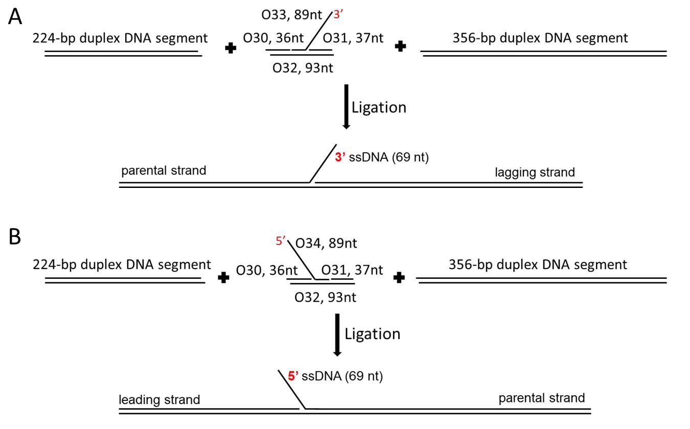
      Figure 1. The assembly process of the fork DNA substrates. A. The F3 DNA substrate: ligate two duplex-DNA segments with sticky ends (the 224-bp segment and the 356-bp segment) and a core fork segment (with a 3'-end, 69-nucleotide single-stranded region) together. B. The F5 DNA substrate: ligate two duplex-DNA segments with sticky ends (the same duplex-DNA segments used for F3) and a core fork segment (with a 5'-end, 69-nucleotide single-stranded region) together.

      
      

      1. Prepare the core segment for the F3 DNA

         1. Phosphorylate each oligonucleotide (O30, O31, O32, O33):

            Add the components to a 1.5 ml microfuge tube and mix well: 10 μl of the oligonucleotide (100 μM), 5 μl of the 10× T4 ligase buffer, 1 μl of the kinase, 34 μl of DDI H₂O. Incubate it at 37 °C for 1 h.

         2. Anneal the oligonucleotides (core segment):

            For F3 fork substrate, add the phosphorylated oligonucleotides (O30, O31, O32, O33) in equimolar ratio to a microtube and mix well. Put the tube in the boiled water bath (~100 °C) and incubate it in the water bath overnight, letting it cool down to room temperature (~20 °C) gradually.

            Note: We usually run ~2 μl sample on an agarose gel (~2%, w/v) to check the annealing product.

      2. Ligate the duplex-DNA segments with the core segment

         Add the segments and the ligase into a microtube: the molar ratio of each segment is 1:1:1.2 (224-bp segment: 356-bp segment: core segment). Incubate it at 16 °C overnight.

         Note: We usually run ~2 μl sample on an agarose gel (~2%, w/v) to check the ligation reaction.

      3. Purify the ligation product by HPLC. Collect the DNA and concentrate the solution using the Amicon Ultra-0.5 ml centrifugal filters (pore size: 30 kDa NMWCO).

      4. Determine the DNA concentration by measuring the absorbance of the purified DNA at 260 nm.

   4. Assemble the F5 DNA substrate (see schematic in Figure 1B)

      1. Prepare the core segment for the F5 DNA

         1. Phosphorylate each oligonucleotide (O30, O31, O32, O34):Add the components to a 1.5 ml microfuge tube and mix well: 10 μl of the oligonucleotide (100 μM), 5 μl of the 10× T4 ligase buffer, 1 μl of the kinase, 34 μl of DDI H₂O. Incubate it at 37 °C for 1 h.

         2. Anneal the oligonucleotides:

            Add the phosphorylated oligonucleotides (O30, O31, O32, O34) in equimolar ratio to a microtube and mix well. Follow the same procedure that was described in 3.a.ii.

            Note: We usually run ~2 μl sample on an agarose gel (~2%, w/v) to check the annealing product.

      2. Ligate the duplex-DNA segments with the core segment: Follow the same procedure that was described in 3.b.

      3. Purify the ligation product by HPLC. Collect the DNA and concentrate the solution using the Amicon Ultra-0.5 ml centrifugal filters (pore size: 30 kDa NMWCO).

      4. Determine the DNA concentration by measuring the absorbance of purified DNA at 260 nm.

         
         

2. Functionalize the mica surface

   1. Prepare a 50 mM 1-(3-Aminopropyl) silatrane APS stock solution in DDI H₂O as described (Shlyakhtenko et al., 2013). The stock solution can be kept for more than a year at 4 °C. Prepare 15 ml of the working APS (167 μM) from the APS stock.

   2. Cut 1 × 3 cm strips of mica from high-quality mica sheets. Check that the piece fits when placed diagonally in a cuvette. A schematic of the process to prepare APS functionalized mica for AFM imaging is shown in Stumme-Diers et al. (2019). Use a razor blade to cleave layers of the mica until both sides are freshly cleaved, and the piece should be thin (~0.1 mm). Immediately place the mica piece into the APS filled cuvette and incubate for 30 min.

   3. Rinse the mica piece under running DDI H₂O droplets or slow fluid for ~10 s. Completely dry both sides of the APS-mica strip under the gentle argon flow.

      Note: Use the lock tweezer to take the mica piece. A non-woven cellulose and polyester wipe (recommended wipe detailed in Materials) can be used to aid in wicking water from the edge of the mica when drying; keep the mica piece perpendicular to the wipe to avoid damage to the functionalized mica surface.

   4. The APS-functionalized mica is ready to use. For storage, place the dry mica strip into a clean cuvette and keep it in a vacuum chamber. The functionalized mica can be stored in the vacuum chamber or in the argon atmosphere for at least a week.

      
      

3. Prepare the protein-DNA complex

   1. Prepare the binding solution from the 10× binding buffer (see Recipes). Take 1 μl of the 10× binding buffer and make up the volume to 10 μl with DDI H₂O. The binding solution contains 10 mM Tris-HCl (pH 7.5), 50 mM NaCl, 5 mM MgCl₂, and 1 mM DTT.

   2. Prepare the Protein-DNA mixture

      1. Prepare the PriA-DNA complex. Mix 3.6 μl of the PriA monomer (molar concentration: 100 nM) with 1 μl of DNA substrate (molar concentration: 45 nM) in a molar ratio of 8:1. Add 5.4 μl of the binding buffer to the mixture and incubate at room temperature (~20 °C) for 10 min.

      2. Prepare the PriA-SSB-DNA complex. Mix 10 μl of the SSB tetramer (molar concentration: 50 nM) with 10 μl of the PriA monomer, and the mixture was kept on ice for 30 minutes before use. Take 3.6 μl of the protein-mixture and add it to the fork DNA substrate in a 1:2:4 (DNA substrates: SSB: PriA) molar ratio. Make up the volume to 10 µl with the binding buffer and incubate the mixture for 10 min at room temperature (~20 °C).

   3. After incubation, dilute the complex-solution to achieve lower DNA concentration (~2 nM), which is ready for deposition onto the APS functionalized mica.

      Note: Arrange the experiment to have the APS-mica ready-to-use before this step. Once the mixture is diluted, it should be immediately deposited onto the mica.

      
      

4. Prepare the protein-DNA samples on the APS-mica

   1. Apply double-faced adhesive tape to several magnetic pucks and place them to the side.

   2. Cut the APS-mica substrate to 1 × 1 cm squares. Place these pieces in a clean petri dish and keep them covered.

   3. Prepare a dilution of the assembled protein-DNA complexes (keep the final DNA concentration at 1.0 to 2.0 nM) using the binding buffer.

   4. Deposit 10 μl of the diluted protein-DNA sample at the center of the APS-mica piece and incubate for two minutes. Gently rinse the sample with DDI H₂O droplets for ~10 s to remove all buffer components.

   5. Dry the deposited sample under a light flow of clean argon gas with the help of a clean wipe. Attach the sample to the magnetic puck and store it in a vacuum cabinet filled with argon for at least 3 h before imaging.

      Note: Be careful not to touch the mica surface after sample deposition.

      
      

5. AFM imaging

   Images were acquired using a MultiMode 8, Nanoscope V system (Bruker, Santa Barbara, CA) operated in tapping mode in the air on TESPA probes (320 kHz nominal frequency and a 42 N/m spring constant) from the same vendor.

   1. Mount the probe into the cantilever holder. Be sure that it is in firm contact with the end of the groove. Mount the cantilever holder onto the end of the scanner head.

   2. Mount the sample on the AFM stage.

      Note: Be careful not to contact the sample surface.

   3. Adjust the laser until the sum is at the maximum so that it is on the cantilever. Adjust the photodetector and set the vertical and lateral deflection values to near zero.

   4. Tune the cantilever. Click 'AutoTune' to find the cantilever's free-air resonant frequency and adjust the peak offset to ~3%.

   5. Set Initial Scan Parameters. Set the initial Scan Size to 1 µm, X and Y Offset to 0, and Scan Angle to 0. Set Integral Gain to 1.0, Proportional Gain to 5, and Scan Rate to 1 Hz. Click the engage button to begin the approach.

   6. Once approached, gradually optimize the Amplitude Setpoint until the surface of the sample is clearly seen. Once the scan parameters are optimized, increase the resolution to 1024 × 1024 pixels. Check to see if Trace and Retrace are tracking each other well during the scan. Click the capture button followed by the engage button to begin image acquisition.

   7. Flatten the image. Click 'Flatten' in the tool panel and save as a copy in the same folder.

   
   

   Notes:

1. AFM calibration is accomplished with the use of a calibration reference and the instruction manual provided by the manufacturer (NanoScope Software Version 5, 004-210-000). According to this protocol, use the Platinum Coated Calibration Grid ( PG ), 1 µm × 1 µm period [100 nm Depth (± 10%)] as the calibration reference and follow the instructions in the manual for the instrument. For Z-axis calibration, by measuring the vertical features of the image using Depth analysis of the same software to correct the Z sensitivity parameter. To accomplish this, divide the actual depth of features (100 nm for PG ) by the measured depth (indicated in Depth analysis by the Peak-to-Peak value), multiply this quotient by the Z sensitivity value in the Z Calibration dialog box, and replace the former Z sensitivity value with the new result.

2. During auto-tuning of the cantilever, the resonance frequency and drive amplitude are automatically selected for the largest signal-to-noise ratio. In our AFM imaging system (MultiMode 8, Nanoscope V system), the drive amplitude is usually 5-15 mV and yields 200-250 mV free amplitude. If needed, the free amplitude (in volts) can be converted to the deflection of the cantilever (in nm) with the calibrated spring constant and inverse optical lever sensitivity of the cantilever, following the detailed instruction provided by the manufacturer (NanoScope Software Version 5, 004-210-000). For the TESPA probe, the nominal spring constant is 37 nN/nm and nominal sensitivity is 60 nm/V, thus nominally, the free amplitude (200-250 mV) is ~12-15 nm.

3. The setpoint values were manually adjusted to the maximal stable values during scanning to maintain the high-resolution image and minimize the tip sweeping effect. The operational amplitude varies on different instruments and or tips. In our AFM imaging system (MultiMode 8, Nanoscope V system), the amplitude setpoint is 150 mV, corresponding to ~80% of the free amplitude of the cantilever.

Data analysis

The AFM images were analyzed using the FemtoScan Online software package (Advanced Technologies Center, Moscow, Russia). Graphs were made by Origin software (OriginLab Corporation, Northampton, MA, USA).

1. Measure the contour length. Open the flattened image in FemtoScan, measure and record the contour length of the free DNA from one end to the other. For the internal length calibration, use the measurements to generate a histogram and fit it with a normal (Gaussian) distribution. To obtain the calibration factor, divide the peak center (Xc) by the substrate length into base pairs.

   Note: The calibration factor should be ~0.34.

2. Measure the position of the protein (Figure 2). Start from the end of the shorter arm on the DNA substrates towards the center of the protein to obtain the position of the protein (arm length 1, shown in Figure 2). Keep recording from the center of the protein towards the other end of the DNA substrate to obtain the contour length of the DNA (arm length 1 and arm length 2 together, shown in Figure 2). Divide each arm length by the calculated calibration factor to obtain arm lengths in DNA base pairs. A histogram for the distribution of the protein can be made from the dataset of arm length 1 (Figure 2C).

   
   

   
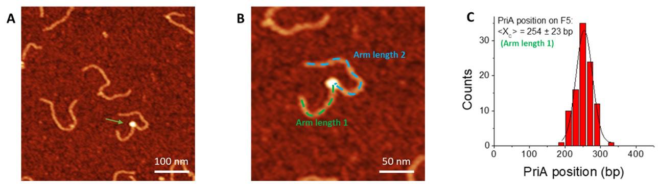
   Figure 2. Measurement of the protein position. A. Representative AFM image (0.5 × 0.5 µm) of F5 with PriA. The Z-scale is 3 nm. Arrow points to bound PriA on the F5 DNA substrate. B. Zoomed-in image (0.25 × 0.25 µm) with the dotted line showing the contour length measurement. The position of each protein is measured from the end of the shorter arm to the center of the protein (dotted green line), and the total length of the protein-bound DNA substrate was measured continuously from the center of the protein to the end of the other arm (dotted blue line). C. Histogram for PriA position on F5 DNA using the data of the short arm length. The histogram was fitted by Gaussian with a single peak centered at 254 ± 23 bp (S.D.), and with a bin size of 20 bp.

   
   

   For the double-feature complexes in the SSB-PriA-DNA results, measure the height of each feature using the cross-section feature of the software as described below, and assign the taller one to SSB. For the length measurement, start from the end closer to the SSB, continuously measure and record towards the center of SSB and PriA, keep on recording until the end of the other side of the DNA substrate. Plot these values as a chart by setting the DNA length as clustered column and protein position as scatter (Figure 3).

   
   

   
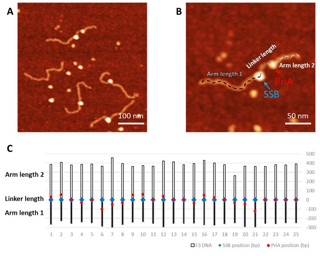
   Figure 3. Measurement of the protein distribution of the complexes containing PriA and SSB proteins. A. Representative AFM image of the PriA+SSB+fork DNA (0.5 × 0.5 µm). The Z-scale is 3 nm. B. The zoomed-in image (0.25 × 0.25 µm) of the double-protein complex with the dotted line showing the contour length measurement. The green arrow directs to PriA in the complex, while the SSB position is directed by the blue arrow. C. Map of the proteins on the F3 DNA substrate with the SSB position corresponding to zero value. Blue squares indicate the position of SSB and the red dots point to the PriA position.

   
   

3. Measure the volume of the protein. For each protein, collect two sets of height (H) and full width at half maximum values (D) from orthogonal cross-section measurements (Figure 4A). Apply the measurements to the formula as described in Gilmore et al. (2009): V = 3.14 × H/6 × (0.75 x D₁ x D₂ + H²). Plot these values as a histogram and fit the peak(s) with a normal (Gaussian) distribution to obtain the volume of the protein population.

   Note: In our AFM-imaging system (MultiMode 8, Nanoscope V system, E scanner), the accuracy of the vertical measurement is at the sub-nm level (Lyubchenko, 2011). The measured height of DNA in the air is usually around 0.6 to 0.8 nm as performed in our and other laboratories (Thomson et al., 1996; Hansma et al., 1996; Maeda et al., 1999; Pietrasanta et al., 1999; Ye et al., 2000; Kato et al., 2002; Shlyakhtenko et al., 2003), and it can be taken as a control for the height measurements of the protein-DNA complexes. Additionally, the measured thickness of the supported phospholipid bilayer is 4-5 nm (Lv et al., 2018), which is in perfect agreement with the bilayer measurements obtained by other methods.

   
   

   
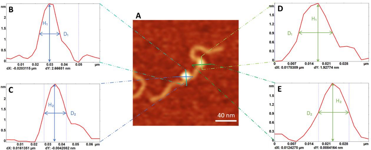
   Figure 4. Measurement of the size of the protein. A. Representative AFM image of the double-protein complex (0.2 × 0.2 µm). Cross-section profiles (green and blue lines) of a protein produce the height distribution curves shown in (B-E): (B) and (C) are the plots for SSB, and (D) and (E) show the height distributions for PriA. From these curves, height (H) and width (D) values are used for calculating the protein volume.

Recipes

1. 10× binding buffer

   100 mM Tris-HCl (pH 7.5)

   500 mM NaCl

   50 mM MgCl₂

   10 mM DTT

Acknowledgments

The work was supported by the National Institutes of Health grants R01 GM118006 to YLL and R01 GM100156 to PRB and YLL. This protocol was adapted from a previously described work (Wang et al., 2020).

Competing interests

There are no competing interests to declare.

References

1. Bhattacharyya, B., George, N. P., Thurmes, T. M., Zhou, R., Jani, N., Wessel, S. R., Sandler, S. J., Ha, T. and Keck, J. L. (2014). Structural mechanisms of PriA-mediated DNA replication restart. Proc Natl Acad Sci U S A 111(4): 1373-1378.
2. Cadman, C. J. and McGlynn, P. (2004). PriA helicase and SSB interact physically and functionally. Nucleic Acids Res 32(21): 6378-6387.
3. Cox, M. M., Goodman, M. F., Kreuzer, K. N., Sherratt, D. J., Sandler, S. J. and Marians, K. J. (2000). The importance of repairing stalled replication forks. Nature 404(6773): 37-41.
4. Gabbai, C. B. and Marians, K. J. (2010). Recruitment to stalled replication forks of the PriA DNA helicase and replisome-loading activities is essential for survival. DNA Repair (Amst) 9(3): 202-209.
5. Gilmore, J. L., Suzuki, Y., Tamulaitis, G., Siksnys, V., Takeyasu, K. and Lyubchenko, Y. L. (2009). Single-molecule dynamics of the DNA-EcoRII protein complexes revealed with high-speed atomic force microscopy. Biochemistry 48(44): 10492-10498.
6. Hansma, H. G., Revenko, I., Kim, K. and Laney, D. E. (1996). Atomic force microscopy of long and short double-stranded, single-stranded and triple-stranded nucleic acids. Nucleic Acids Res 24(4): 713-720.
7. Kato, M., McAllister, C. J., Hokabe, S., Shimizu, N. and Lyubchenko, Y. L. (2002). Structural heterogeneity of pyrimidine/purine-biased DNA sequence analyzed by atomic force microscopy. Eur J Biochem 269(15): 3632-3636.
8. Kogoma, T. (1997). Stable DNA replication: interplay between DNA replication, homologous recombination, and transcription. Microbiol Mol Biol Rev 61(2): 212-238.
9. Lv, Z., Banerjee, S., Zagorski, K. and Lyubchenko, Y. L. (2018). Supported Lipid Bilayers for Atomic Force Microscopy Studies. Methods Mol Biol 1814: 129-143.
10. Lyubchenko, Y. L. (2011). Preparation of DNA and nucleoprotein samples for AFM imaging. Micron 42(2): 196-206.
11. Maeda, Y., Matsumoto, T. and Kawai, T. (1999). Observation of single-and double-stranded DNA using non-contact atomic force microscopy.App Sur Sci 140(3-4): 400-405.
12. McGlynn, P. and Lloyd, R. G. (2002). Recombinational repair and restart of damaged replication forks. Nat Rev Mol Cell Biol 3(11): 859-870.
13. Michel, B., Grompone, G., Flores, M. J. and Bidnenko, V. (2004). Multiple pathways process stalled replication forks. Proc Natl Acad Sci U S A 101(35): 12783-12788.
14. Michel, B., Sinha, A. K. and Leach, D. R. F. (2018). Replication Fork Breakage and Restart in Escherichia coli. Microbiol Mol Biol Rev 82(3): e00013-18.
15. Pietrasanta, L. I., Thrower, D., Hsieh, W., Rao, S., Stemmann, O., Lechner, J., Carbon, J. and Hansma, H. (1999). Probing the Saccharomyces cerevisiae centromeric DNA (CEN DNA)-binding factor 3 (CBF3) kinetochore complex by using atomic force microscopy. Proc Natl Acad Sci U S A 96(7): 3757-3762.
16. Sandler, S. J. and Marians, K. J. (2000). Role of PriA in replication fork reactivation in Escherichia coli. J Bacteriol 182(1): 9-13.
17. Shlyakhtenko, L. S., Gall, A. A. and Lyubchenko, Y. L. (2013). Mica functionalization for imaging of DNA and protein-DNA complexes with atomic force microscopy.Methods Mol Biol 931: 295-312.
18. Shlyakhtenko, L. S., Gall, A. A., Filonov, A., Cerovac, Z., Lushnikov, A. and Lyubchenko, Y. L. (2003). Silatrane-based surface chemistry for immobilization of DNA, protein-DNA complexes and other biological materials. Ultramicroscopy 97(1-4): 279-287.
19. Stumme-Diers, M. P., Stormberg, T., Sun, Z. and Lyubchenko, Y. L. (2019). Probing The Structure And Dynamics Of Nucleosomes Using Atomic Force Microscopy Imaging. J Vis Exp(143). doi: 10.3791/58820.
20. Thomson, N. H., Kasas, S., Smith, B., Hansma, H. G. and Hansma, P. K. (1996). Reversible binding of DNA to mica for AFM imaging. Langmuir 12(24): 5905-5908.
21. Wang, Y., Sun, Z., Bianco, P.R. and Lyubchenko, Y.L. (2020). Atomic force microscopy–based characterization of the interaction of PriA helicase with stalled DNA replication forks. J Biol Chem 295(18): 6043-6052.
22. Wickner, S. and Hurwitz, J. (1975). Association of phiX174 DNA-dependent ATPase activity with an Escherichia coli protein, replication factor Y, required for in vitro synthesis of phiX174 DNA.Proc Natl Acad Sci U S A 72(9): 3342-3346.
23. Windgassen, T. A., Leroux, M., Sandler, S. J. and Keck, J. L. (2019). Function of a strand-separation pin element in the PriA DNA replication restart helicase. J Biol Chem 294(8): 2801-2814.
24. Windgassen, T. A., Leroux, M., Satyshur, K. A., Sandler, S. J. and Keck, J. L. (2018a). Structure-specific DNA replication-fork recognition directs helicase and replication restart activities of the PriA helicase. Proc Natl Acad Sci U S A 115(39): E9075-E9084.
25. Windgassen, T. A., Wessel, S. R., Bhattacharyya, B. and Keck, J. L. (2018b). Mechanisms of bacterial DNA replication restart. Nucleic Acids Res 46(2): 504-519.
26. Ye, J. Y., Umemura, K., Ishikawa, M. and Kuroda, R. (2000). Atomic force microscopy of DNA molecules stretched by spin-coating technique.Anal Biochem 281(1): 21-25.
27. Yu, C., Tan, H. Y., Choi, M., Stanenas, A. J., Byrd, A. K., K, D. R., Cohan, C. S. and Bianco, P. R. (2016). SSB binds to the RecG and PriA helicases in vivo in the absence of DNA. Genes Cells 21(2): 163-184.
28. Zavitz, K. H. and Marians, K. J. (1992). ATPase-deficient mutants of the Escherichia coli DNA replication protein PriA are capable of catalyzing the assembly of active primosomes. J Biol Chem 267(10): 6933-6940.

1. Wang, Y., Sun, Z., Bianco, P. R. and Lyubchenko, Y. L. (2021). Characterize the Interaction of the DNA Helicase PriA with the Stalled DNA Replication Fork Using Atomic Force Microscopy. Bio-protocol 11(5): e3940. DOI: 10.21769/BioProtoc.3940.
   
2. Wang, Y., Sun, Z., Bianco, P.R. and Lyubchenko, Y.L. (2020). Atomic force microscopy–based characterization of the interaction of PriA helicase with stalled DNA replication forks. J Biol Chem 295(18): 6043-6052.