- Protocols

- Articles and Issues
- For Authors
- About
- Become a Reviewer

Investigating the Shape of the Shoot Apical Meristem in Bamboo Using a Superellipse Equation

Published: Vol 7, Iss 23, Dec 5, 2017 DOI: 10.21769/BioProtoc.2644 Views: 6341
Reviewed by: Scott A M McAdamTamara VellosilloSriema L. Walawage
Original research article
The authors used this protocol in:

Apr 2016
Advertisement


Protocol Collections
Comprehensive collections of detailed, peer-reviewed protocols focusing on specific topics


Abstract
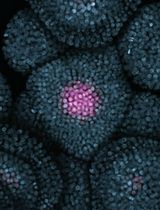
The shoot apical meristem is the origin of bamboo wood. Its structure and morphology are important for maintaining the normal development of bamboo wood. However, the traditional method to describe the morphology of the shoot apical meristem in bamboo or other plants only depends on qualitative approaches. Here we present a protocol for precisely describing the morphology of bamboo shoot apical meristem, which is adapted from our recently published papers (Shi et al., 2015; Wei et al., 2017).
Keywords: BambooBackground
Shoot apical meristem is the source of above-ground tissues. For a long time, its morphology description has been lack of a quantitative method for morphological analysis. This protocol provides a method for better description of the outer contour of the shoot apical meristem of bamboo.
Materials and Reagents
- Completed paraffin sections with plant shoot apical meristem (Wei et al., 2017)
Equipment
- Leica DM2500 light microscope (Germany) (Leica Microsystems, model: Leica DM2500 )
Software
- Windows 7 Operation System (64 bit)
- Photoshop CS6 (Adobe, USA)
- R (ver. 3.3.0)
- MATLAB (ver. R2015b)
- Notepad++ (ver. 7.4.2)
- R and MATLAB scripts (see the Supplementary files)
Procedure
- The images of plant shoot apical meristem are first obtained under a DM2500 light microscope with 40-fold objective lens, and saved as BMP file using default parameters, usually the DPI of the image should be ≥ 72.
- Then the BMP file is opened by Photoshop CS6, and straightened by ‘Image Rotation’ function as shown in Figure 1.
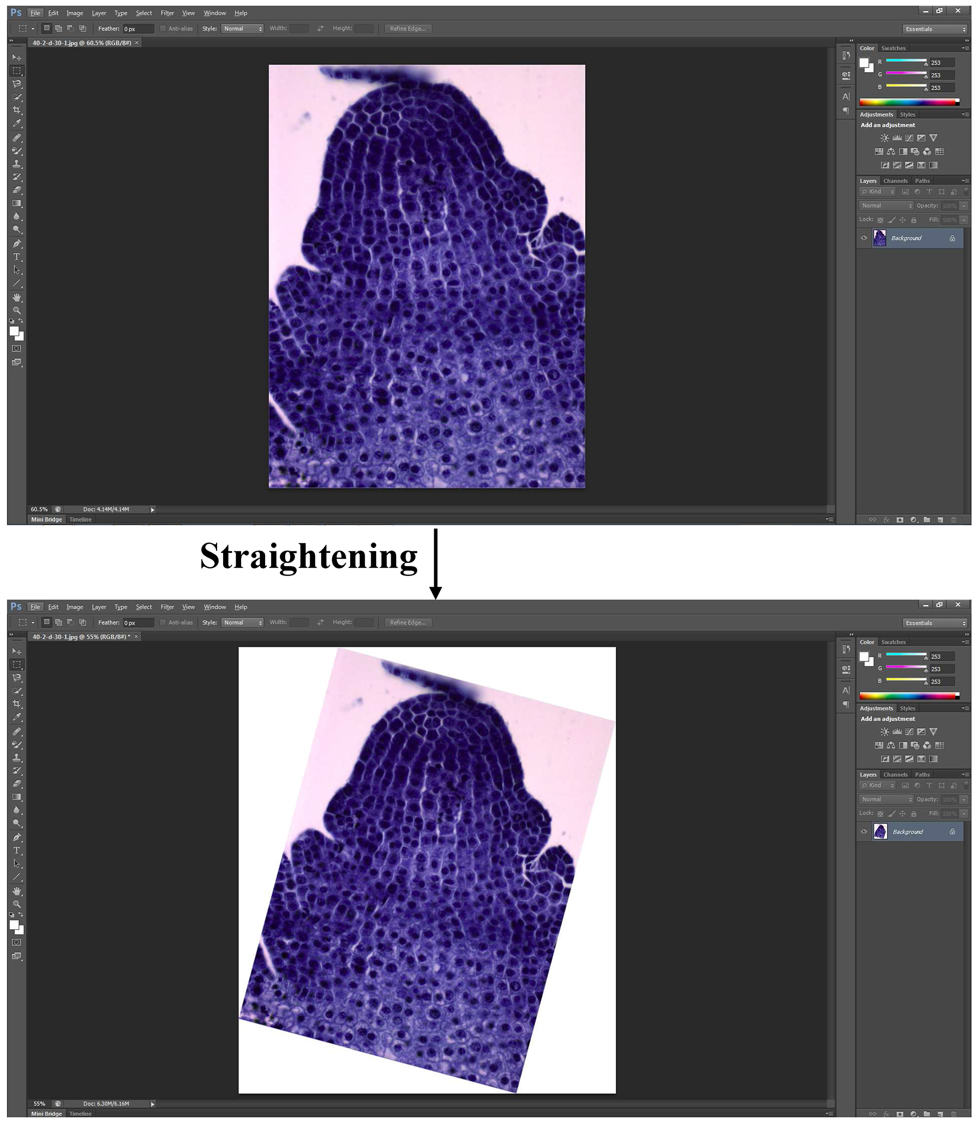
Figure 1. Straightening picture via ‘Image Rotation’ - A line which is parallel with the horizontal axis is added to connect the part just above the first leaf primordium and its corresponding part in another side using the ‘Line tool’ (Figure 2).
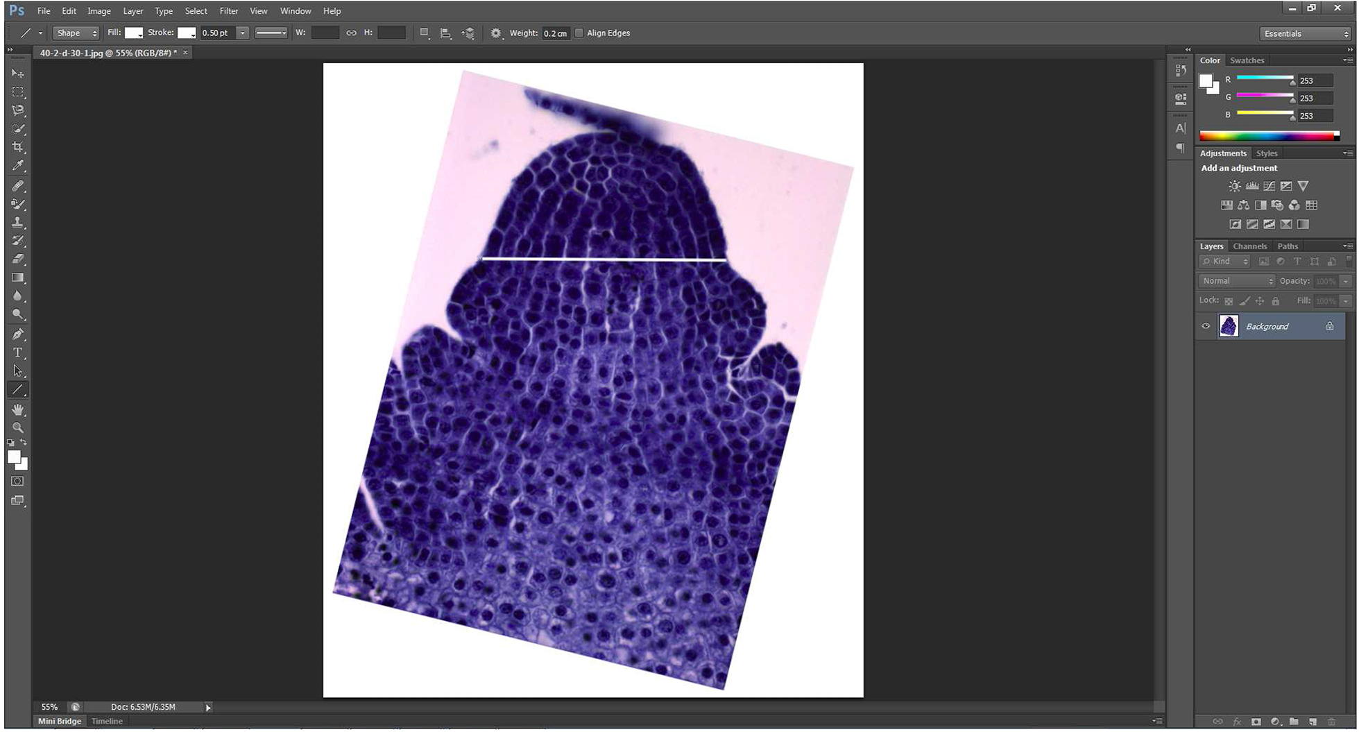
Figure 2. A line just above the first leaf primordium is added - The line and the picture are merged to form a merged picture using the function ‘Layer’ → ‘Merge Visible’.
- The merged picture containing the shoot apical meristem and the straight line is then extracted by ‘Magnetic Lasso Tool’ which is great for following the edges of an object. And they are copied to a new blank layer directly generated by ‘Control + N’ (Figure 3).
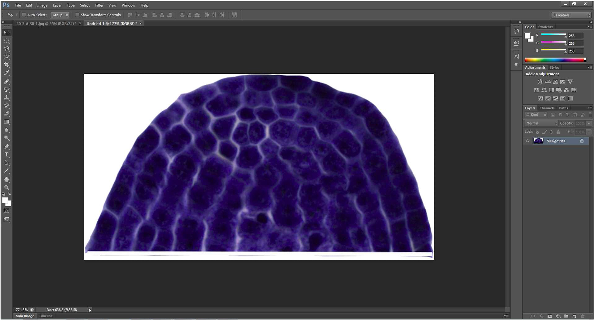
Figure 3. Extracted shoot apical meristem - To duplicate the resulting image, the new generated picture is then flipped by the command combination of ‘Image → Image Rotation → Flip canvas Vertical’ (Figure 4A) to produce a new vertical symmetric picture (Figure 4B).
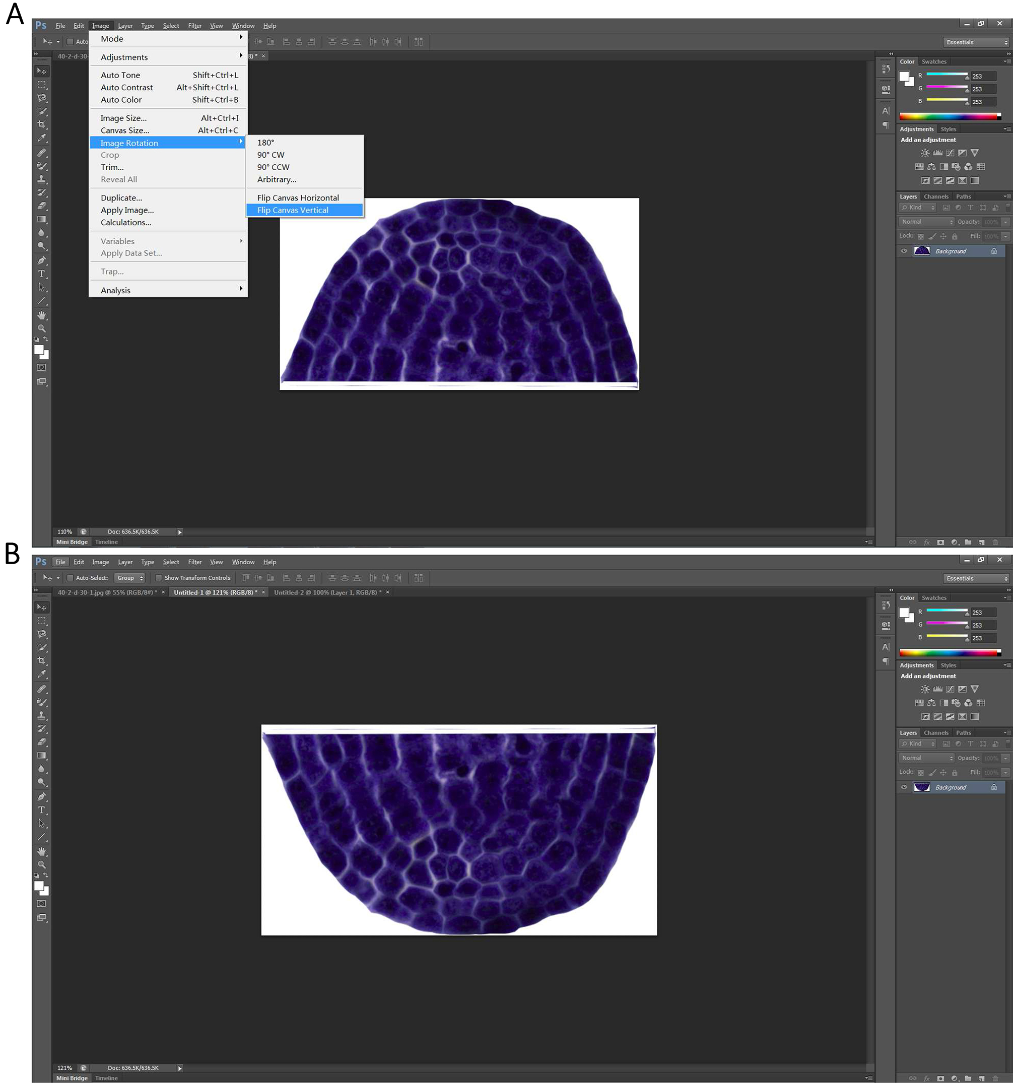
Figure 4. Producing a new vertical symmetric picture of the extracted shoot apical meristem - A new blank layer with the size at least could contain two of the extracted shoot apical meristem is first generated by command ‘Control + N’. The shoot apical meristem and its newly produced vertical symmetric picture are then put together (Figure 5A), and merged using the function ‘Layer’→ ‘Merge Visible’ (Figure 5B).
Note: Before merging the two images, move the two images to get close to each other until there is only a thin line space left between the two images (Figure 5B).
Figure 5. A new picture consisted of the extracted apical meristem and its vertical symmetric image is formed - The merged picture is then extracted by ‘Magnetic Lasso Tool’, and is copied to a new blank layer automatically generated by ‘Control + N’ to make the extracted picture be included by the smallest rectangle (white) in the image (Figure 6).
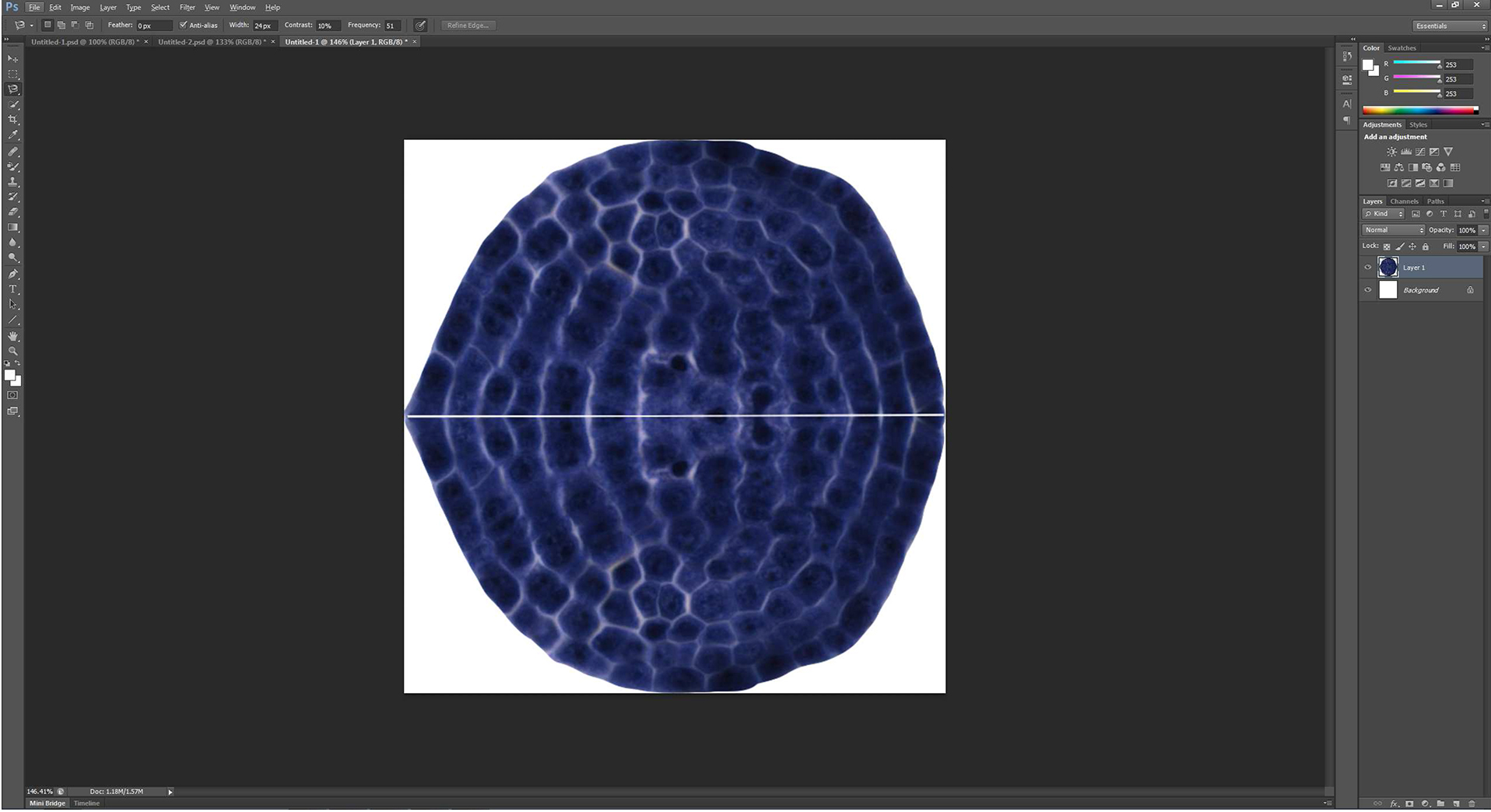
Figure 6. The picture showed in Figure 5B is put in the smallest rectangle
Note: The image boundary is exactly the smallest rectangle that includes the outermost boundary of the combined picture. - The merged picture is then selected by ‘Magnetic Lasso Tool’ (Figure 7A), and is filled by a new solid black layer (Figure 7B) by the command combination of ‘Layer → New fill layer → Solid Color’.
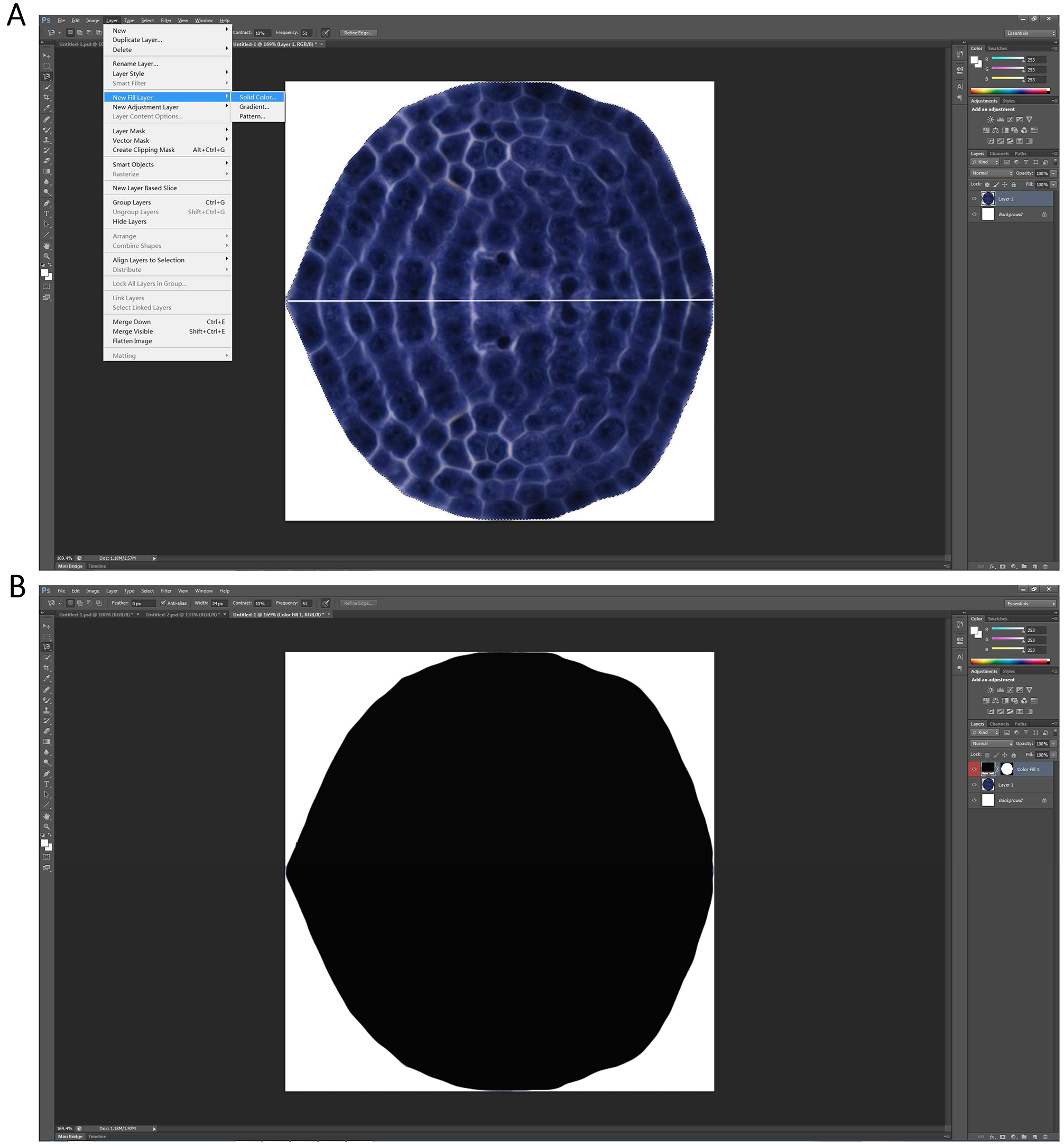
Figure 7. The image showed in Figure 6 is filled by a new solid black layer - The new resulting picture is saved as a BMP file named ‘SF’ in the work directory. Here the directory is ‘I:\Biotool’.
- Open ‘MATLAB’, and change the initial directory to your work directory, and build a subdirectory under your work directory, ‘Scripts’ for example here (Figure 8).
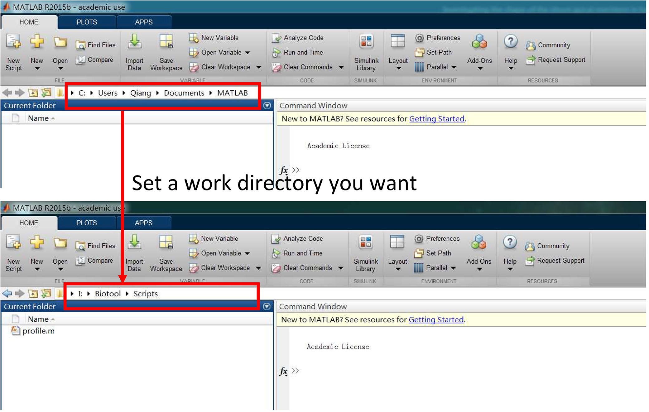
Figure 8. Set a work directory - Put MATLAB script, ‘profile.m’ (Supplementary files) under the ‘Scripts’ directory, and carry out the “profile” on the command line as follows (Shi et al., 2015):
profile (1, 1, 'I:\Biotool\SF.bmp', 'I:\Biotool\edge_data.csv')
After running the script, the user can obtain a ‘.csv’ file under the directory ‘I:\Biotool\’ named ‘edge_data’ which has stored the planar coordinates of the ‘SF’ picture boundary (Figure 9A). The user can also obtain the figure based on the extracted boundary as shown in Figure 9B.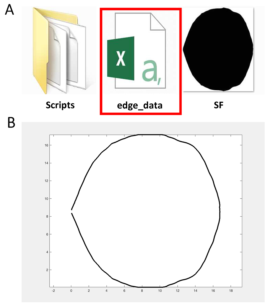 Figure 9. ‘edge_data’ (red rectangle) which has stored the planar coordinates of the picture (A) and the figure based on the extracted boundary (B) are obtained in this step
 - Put ‘R’ scripts which are developed by Shi et al. (2015) basing on the superellipse equation proposed by Gielis (2003), ‘fit.sf.R’ (Shi et al., 2015), ‘optim.sf.R’ (Shi et al., 2015) and ‘simu.sf.R’ (Shi et al., 2015) under the ‘Scripts’ directory (Supplementary files). And open ‘fit.sf.R’, ‘optim.sf.R’ and ‘simu.sf.R’ via Notepad++. Change the directories indicated by the red arrows to your own directory (Figure 10).
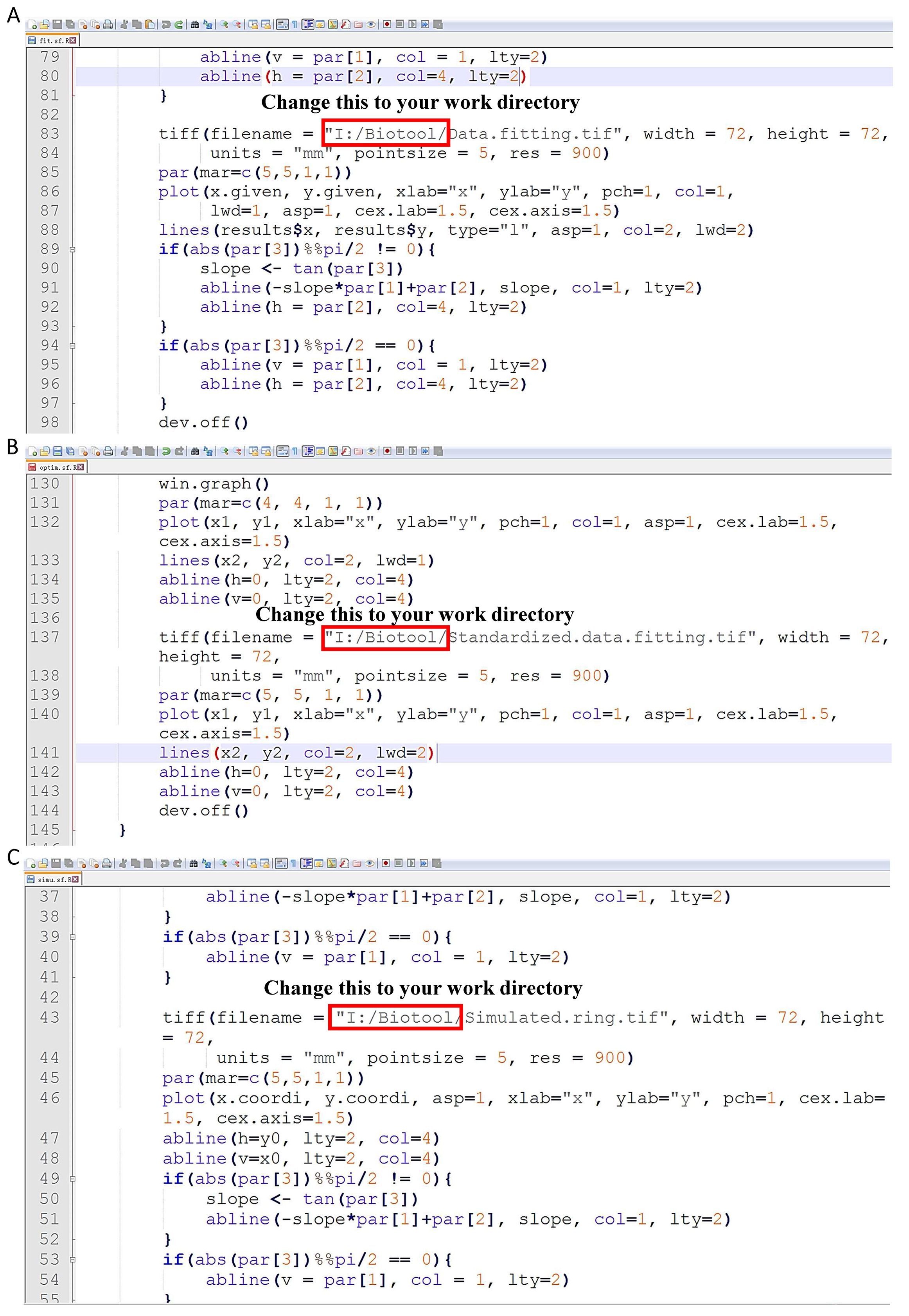
Figure 10. Change the directories indicated by the red arrows in ‘fit.sf.R’ (A), ‘optim.sf.R’ (B) and ‘simu.sf.R’ (C) to your own directory - Open ‘R’ function, and paste the following codes in the console (For more information about those codes, please see the Supplementary file, Appendix S2 of the published paper of Shi et al. (2015) (http://journal.frontiersin.org/article/10.3389/fpls.2015.00856/full):wd <- c("I:/Biotool/Scripts/")
source (paste (wd, "simu.sf.R", sep=""))
source (paste (wd, "optim.sf.R", sep=""))
source (paste (wd, "fit.sf.R", sep=""))
source (paste (wed, "area.sf.R", sep=""))
data <- read.csv ("I:/Biotool/edge_data.csv", header=F)
x.provi <- data [,1]
y.provi <- data[,2]
x0.val <- 200
y0.val <- 200
theta.val <- pi/4
a.val <- 50
k.val <- 0.95
n.val <- 1.90
Phi <- seq(0, 2*pi, len=1000)
Para <- c (x0.val, y0.val, theta.val, a.val, k.val, n.val)
CV.val <- 0.01
res1 <- simu.sf(phi=Phi, par=Para, CV=CV.val, fig.opt = F)
x.simu <- res1$x
y.simu <- res1$y
x.width <- range(x.provi)[2] - range(x.provi)[1]
y.width <- range(y.provi)[2] - range(y.provi)[1]
a.ini <- max (y.width, x.width)/2
x0.ini <- (min(x.provi) + max(x.provi))/2
y0.ini <- (min(y.provi) + max(y.provi))/2
theta.ini <- pi/4
k.ini <- 0.95
n.ini <- 1.90
res2 <- optim.sf(x.provi, y.provi, x0.ini, y0.ini, theta.ini, a.ini, k.ini,
n.ini, fig.opt="F", para.list="F", convergence="Chi.square")
x0. range <- x0.ini
y0. range <- y0.ini
theta.range <- seq(0, pi/2, by=pi/8)
a.range <- a.ini
k.range <- seq(0.8, 1, by=0.1)
n.range <- seq(1.8, 2.2, by=0.1)
res3 <- fit.sf(x.provi, y.provi, x0=x0.range, y0=y0.range,
theta=theta.range, a=a.range, k=k.range, n=n.range,
para.list=F, fig.opt=F, convergence="Chi.square")
res4 <- fit.sf(x.provi, y.provi, res3$par[1], res3$par[2],
res3$par [3], res3$par [4], res3$par [5], res3$par [6],
para.list=T, fig.opt=T, convergence="Chi.square")
After the performing, it will finally generate a picture named ‘Data.fitting’ (Figure 11). The solid dark line represents the observed out contour of the two combined shoot apical meristems; the red solid line represents the predicted ring. The dark dashed line represents the direction of major axis; the blue dashed line represents the direction of x-axis. And their theta which indicates the angle value between the dark dashed line and the blue dashed line was calculated and displayed in R console (Figure 12).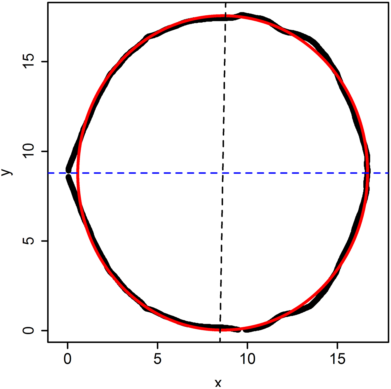
Figure 11. The predicted image of the picture showed in Figure 7A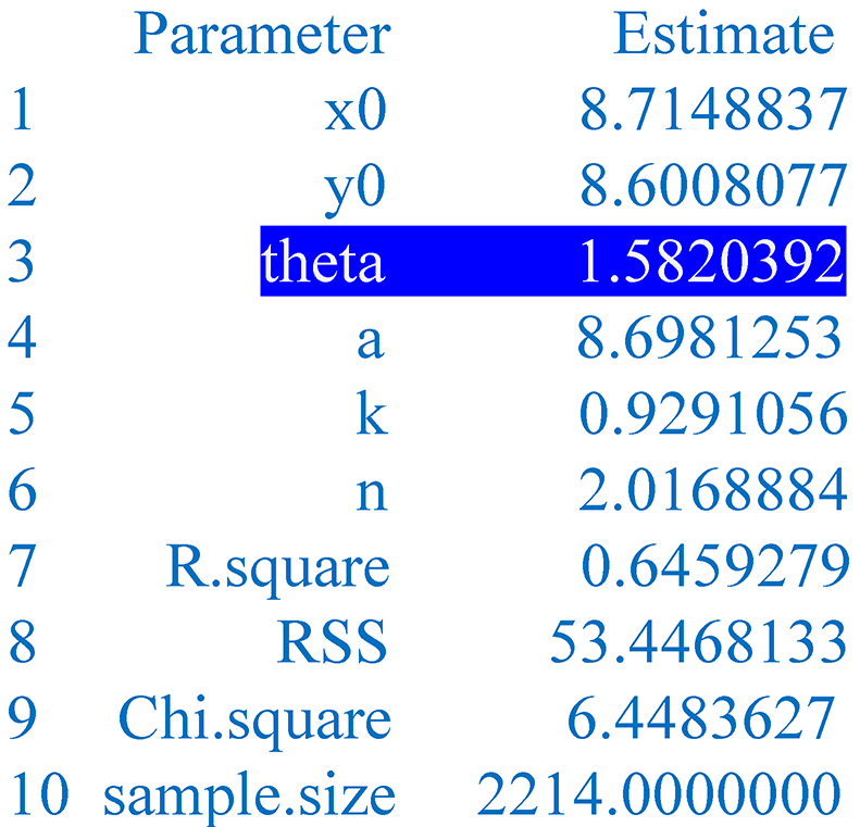
Figure 12. Parameters of the predicted image. The given parameters include the abscissa and ordinate of the pole (x0, y0) in the Cartesian system, the angle theta between the major axis and the x-axis, the major semi-axis a, the ratio k of the minor semi-axis (b) to the major semi-axis (a), the power n, the coefficient of determination (R.square), the χ2 (Chi.square) or the residual sum of squares (RSS).
Data analysis
For more information about the scripts’ function, please see the Supplementary file, data sheet 2 of the published paper of Shi et al. (2015) (http://journal.frontiersin.org/article/10.3389/fpls. 2015.00856/full). Here we also provide an example for using the protocol to compare the morphology of the shoot apical meristems (SAM) between Moso bamboo shoot and its thick wall variant at different developmental stage (Figure 13). In this example, by using the mathematical modeling, we found that the SAM morphology of the thick wall Moso bamboo shoot is flatter than the wild type Moso (Figure 13).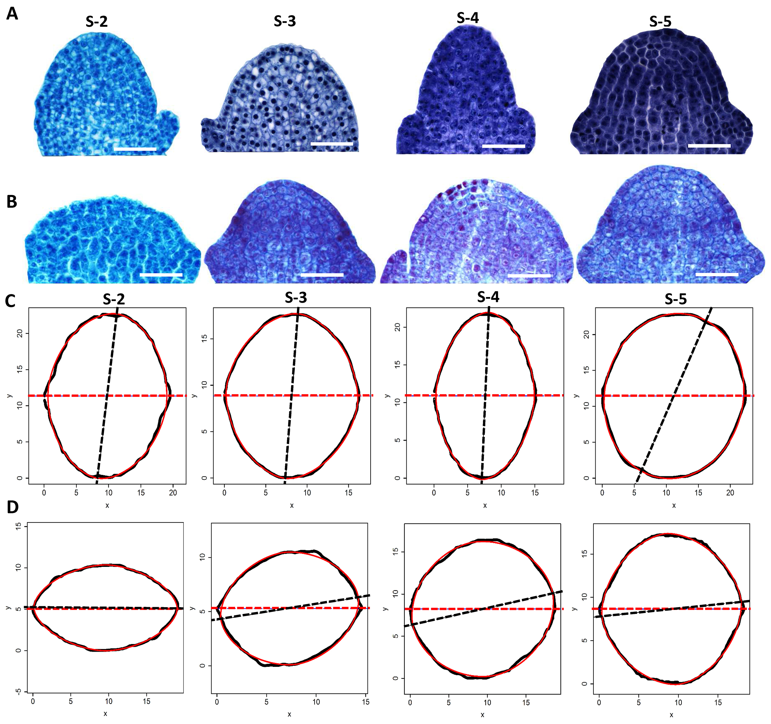
Figure 13. SAMs comparisons between the thick wall Moso and its corresponding wild type using the protocol presented here (Wei et al., 2017). Morphology of apical meristems of the thick wall Moso (A) and wild type Moso (B) bamboo shoots at different developmental stages (S2 to S6). Outlines of the apical meristem of the wild type Moso (C) and the thick wall variant (D) (black solid lines) and the predicted outlines using superellipse equation (red solid lines) at different developmental stages (from S-2 to S-5). Each outline was combined by two corresponding semi-outlines of the apical meristem. The dark dashed line represents the direction of major axis and the red dashed line represents the direction of x-axis. Scale bars = 50 μm.
Acknowledgments
This study was supported in part by Natural Science Foundation of China (grant Nos. 31670602 and 31301808) (to W.Q.), a project funded by the Priority Academic Program Development of Jiangsu Higher Education Institutions. The protocol was adapted from previous work (Shi et al., 2015; Wei et al., 2017). The authors declare no conflicts of interest or competing interests that may impact the design and implementation of this protocol.
References
- Gielis, J. (2003). A generic geometric transformation that unifies a wide range of natural and abstract shapes. Am J Bot 90(3): 333-338.
- Shi, P. J., Huang, J. G., Hui, C., Grissino-Mayer, H. D., Tardif, J. C., Zhai, L. H., Wang, F. S. and Li, B. L. (2015). Capturing spiral radial growth of conifers using the superellipse to model tree-ring geometric shape. Front Plant Sci 6: 856.
- Wei, Q., Jiao, C., Guo, L., Ding, Y., Cao, J., Feng, J., Dong, X., Mao, L., Sun, H., Yu, F., Yang, G., Shi, P., Ren, G. and Fei, Z. (2017). Exploring key cellular processes and candidate genes regulating the primary thickening growth of Moso underground shoots. New Phytol 214(1): 81-96.
Article Information
Copyright
© 2017 The Authors; exclusive licensee Bio-protocol LLC.
How to cite
Wei, Q. and Shi, P. (2017). Investigating the Shape of the Shoot Apical Meristem in Bamboo Using a Superellipse Equation. Bio-protocol 7(23): e2644. DOI: 10.21769/BioProtoc.2644.
Category
Plant Science > Plant developmental biology > General
Cell Biology > Tissue analysis > Tissue imaging
Do you have any questions about this protocol?
Post your question to gather feedback from the community. We will also invite the authors of this article to respond.